SC IV G. Statistical Analysis of Results of Biological Assays and Tests
Contents
1. INTRODUCTION
1.1. General design and precision
2. RANDOMISATION AND INDEPENDENCE OF INDIVIDUAL TREATMENTS
3. ASSAYS DEPENDING UPON QUANTITATIVE RESPONSES
3.1. Statistical models
3.1.1. General principles
3.1.2. Routine assays
3.1.3. Calculations and restrictions
3.2. The parallel-line model
3.2.1. Introduction
3.2.2. Assay design
3.2.2.1. Completely randomised design
3.2.2.2. Randomised block design
3.2.2.3. Latin square design
3.2.2.4. Cross-over design
3.2.3. Analysis of variance
3.2.4. Tests of validity
3.2.5. Estimation of potency and confidence limits
3.2.6. Missing values
3.3. The slope-ratio model
3.3.1. Introduction
3.3.2. Assay design
3.3.3. Analysis of variance
3.3.3.1. The (hd + 1)-design
3.3.3.2. The (hd)-design
3.3.4. Tests of validity
3.3.5. Estimation of potency and confidence limits
3.3.5.1. The (hd + 1)-design
3.3.5.2. The (hd)-design
3.4 Extended sigmoid dose-response curves
4. ASSAYS DEPENDING UPON QUANTAL RESPONSES
4.1. Introduction
4.2. The probit method
4.2.1. Tabulation of the results
4.2.2. Tests of validity
4.2.3. Estimation of potency and confidence limits
4.2.4. Invalid assays
4.3. The logit method
4.4. Other shapes of the curve
4.5. The median effective dose
5. EXAMPLES
5.1. Parallel-line model
5.1.1. Two-dose multiple assay with completely randomised design
5.1.2. Three-dose Latin square design
5.1.3. Four-dose randomised block design
5.1.4. Five-dose multiple assay with completely randomised design
5.1.5. Twin cross-over design
5.2. Slope-ratio model
5.2.1. A completely randomised (0,3,3)-design
5.2.2. A completely randomised (0,4,4,4)-design
5.3. Quantal responses
5.3.1. Probit analysis of a test preparation against a reference
5.3.2. Logit analysis and other types of analysis of a test preparation against a reference
5.3.3. The ED50 determination of a substance using the probit method
5.4. Extended sigmoid dose-response curves
5.4.1. Four-parameter logistic curve analysis
6. COMBINATION OF ASSAY RESULTS
6.1. Introduction
6.2. Weighted combination of assay results
6.2.1. Calculation of weighting coefficients
6.2.2. Homogeneity of potency estimates
6.2.3. Calculation of the weighted mean and confidence limits
6.2.4. Weighted mean and confidence limits based on the intra- and inter-assay variation
6.3. Unweighted combination of assay results
6.4. Example of a weighted mean potency with confidence limits
7. BEYOND THIS ANNEX
7.1. General linear models
7.2. Heterogeneity of variance
7.3. Outliers and robust methods
7.4. Correlated errors
7.5. Extended non-linear dose-response curves
7.6 Non-parallelism of dose-response curves
8. TABLES AND GENERATING PROCEDURES
8.1. The F-distribution
8.2. The t-distribution
8.3. The χ2-distribution
8.4. The Φ-distribution
8.5. Random permutations
8.6. Latin squares
9. GLOSSARY OF SYMBOLS
10. LITERATURE
1. Introduction
This chapter provides guidance for the design of bioassays prescribed in the European Pharmacopoeia (Ph. Eur.) and for analysis of their results. It is intended for use by those whose primary training and responsibilities are not in statistics, but who have responsibility for analysis or interpretation of the results of these assays, often without the help and advice of a statistician. The methods of calculation described in this annex are not mandatory for the bioassays which themselves constitute a mandatory part of the Ph. Eur. Alternative methods can be used and may be accepted by the competent authorities, provided that they are supported by relevant data and justified during the assay validation process. A wide range of computer software is available and may be useful depending on the facilities available to, and the expertise of, the analyst.
Professional advice should be obtained in situations where: a comprehensive treatment of design and analysis suitable for research or development of new products is required; the restrictions imposed on the assay design by this chapter are not satisfied, for example particular laboratory constraints may require customized assay designs, or equal numbers of equally spaced doses may not be suitable; analysis is required for extended non-linear dose-response curves, for example as may be encountered in immunoassays. An outline of extended dose-response curve analysis for one widely used model is nevertheless included in Section 3.4 and a simple example is given in Section 5.4.
1.1. General design and precision
Biological methods are described for the assay of certain substances and preparations whose potency cannot be adequately assured by chemical or physical analysis. The principle applied wherever possible throughout these assays is that of comparison with a standard preparation so as to determine how much of the substance to be examined produces the same biological effect as a given quantity, the Unit, of the standard preparation. It is an essential condition of such methods of biological assay that the tests on the standard preparation and on the substance to be examined be carried out at the same time and under identical conditions.
For certain assays (determination of virus titre for example) the potency of the test sample is not expressed relative to a standard. This type of assay is dealt with in Section 4.5.
Any estimate of potency derived from a biological assay is subject to random error due to the inherent variability of biological responses and calculations of error should be made, if possible, from the results of each assay, even when the official method of assay is used. Methods for the design of assays and the calculation of their errors are, therefore, described below. In every case, before a statistical method is adopted, a preliminary test is to be carried out with an appropriate number of assays, in order to ascertain the applicability of this method.
The confidence interval for the potency gives an indication of the precision with which the potency has been estimated in the assay. It is calculated with due regard to the experimental design and the sample size. The 95 per cent confidence interval is usually chosen in biological assays. Mathematical statistical methods are used to calculate these limits so as to warrant the statement that there is a 95 per cent probability that these limits include the true potency. Whether this precision is acceptable to the European Pharmacopoeia depends on the requirements set in the monograph for the preparation concerned.
The terms “mean” and “standard deviation” are used here as defined in most current textbooks of biometry.
The terms “stated potency” or “labelled potency”, “assigned potency”, “assumed potency”, “potency ratio” and “estimated potency” are used in this section to indicate the following concepts:
Section 9 (Glossary of symbols) is a tabulation of the more important uses of symbols throughout this annex. Where the text refers to a symbol not shown in this section or uses a symbol to denote a different concept, this is defined in that part of the text.
2. Randomisation and independence of individual treatments
The allocation of the different treatments to different experimental units (animals, tubes, etc.) should be made by some strictly random process. Any other choice of experimental conditions that is not deliberately allowed for in the experimental design should also be made randomly. Examples are the choice of positions for cages in a laboratory and the order in which treatments are administered. In particular, a group of animals receiving the same dose of any preparation should not be treated together (at the same time or in the same position) unless there is strong evidence that the relevant source of variation (for example, between times, or between positions) is negligible. Random allocations may be obtained from computers by using the built-in randomisation function. The analyst must check whether a different series of numbers is produced every time the function is started.
The preparations allocated to each experimental unit should be as independent as possible. Within each experimental group, the dilutions allocated to each treatment are not normally divisions of the same dose, but should be prepared individually. Without this precaution, the variability inherent in the preparation will not be fully represented in the experimental error variance. The result will be an under-estimation of the residual error leading to:
1) an unjustified increase in the stringency of the test for the analysis of variance (see Sections 3.2.3 and 3.2.4),
2) an under-estimation of the true confidence limits for the test, which, as shown in Section 3.2.5, are calculated from the estimate of s2, the residual error mean square.
3. Assays depending upon quantitative responses
3.1. STATISTICAL MODELS
3.1.1. General principles
The bioassays included in the Ph. Eur. have been conceived as “dilution assays”, which means that the unknown preparation to be assayed is supposed to contain the same active principle as the standard preparation, but in a different ratio of active and inert components. In such a case the unknown preparation may in theory be derived from the standard preparation by dilution with inert components. To check whether any particular assay may be regarded as a dilution assay, it is necessary to compare the dose-response relationships of the standard and unknown preparations. If these dose-response relationships differ significantly, then the theoretical dilution assay model is not valid. Significant differences in the dose-response relationships for the standard and unknown preparations may suggest that one of the preparations contains, in addition to the active principle, other components which are not inert but which influence the measured responses.
To make the effect of dilution in the theoretical model apparent, it is useful to transform the dose-response relationship to a linear function on the widest possible range of doses. 2 statistical models are of interest as models for the bioassays prescribed: the parallel-line model and the slope-ratio model.
The application of either is dependent on the fulfilment of the following conditions:
1) the different treatments have been randomly assigned to the experimental units,
2) the responses to each treatment are normally distributed,
3) the standard deviations of the responses within each treatment group of both standard and unknown preparations do not differ significantly from one another.
When an assay is being developed for use, the analyst has to determine that the data collected from many assays meet these theoretical conditions.
When conditions 2 and/or 3 are not met, a transformation of the responses may bring a better fulfilment of these conditions. Examples are ln y,  , y2.
, y2.
is useful when the observations follow a Poisson distribution i.e. when they are obtained by counting.For some assays depending on quantitative responses, such as immunoassays or cell-based in vitro assays, a large number of doses is used. These doses give responses that completely span the possible response range and produce an extended non-linear dose-response curve. Such curves are typical for all bioassays, but for many assays the use of a large number of doses is not ethical (for example, in vivo assays) or practical, and the aims of the assay may be achieved with a limited number of doses. It is therefore customary to restrict doses to that part of the dose-response range which is linear under suitable transformation, so that the methods of Sections 3.2 or 3.3 apply. However, in some cases analysis of extended dose-response curves may be desirable. An outline of one model which may be used for such analysis is given in Section 3.4 and a simple example is shown in Section 5.4.
There is another category of assays in which the response cannot be measured in each experimental unit, but in which only the fraction of units responding to each treatment can be counted. This category is dealt with in Section 4.
3.1.2. Routine assays
When an assay is in routine use, it is seldom possible to check systematically for conditions 1 to 3, because the limited number of observations per assay is likely to influence the sensitivity of the statistical tests. Fortunately, statisticians have shown that, in symmetrical balanced assays, small deviations from homogeneity of variance and normality do not seriously affect the assay results. The applicability of the statistical model needs to be questioned only if a series of assays shows doubtful validity. It may then be necessary to perform a new series of preliminary investigations as discussed in Section 3.1.1.
Two other necessary conditions depend on the statistical model to be used:
4A) the relationship between the logarithm of the dose and the response can be represented by a straight line over the range of doses used,
5A) for any unknown preparation in the assay the straight line is parallel to that for the standard.
4B) the relationship between the dose and the response can be represented by a straight line for each preparation in the assay over the range of doses used,
5B) for any unknown preparation in the assay the straight line intersects the y-axis (at zero dose) at the same point as the straight line of the standard preparation (i.e. the response functions of all preparations in the assay must have the same intercept as the response function of the standard).
Conditions 4A and 4B can be verified only in assays in which at least 3 dilutions of each preparation have been tested. The use of an assay with only 1 or 2 dilutions may be justified when experience has shown that linearity and parallelism or equal intercept are regularly fulfilled.
After having collected the results of an assay, and before calculating the relative potency of each test sample, an analysis of variance is performed, in order to check whether conditions 4A and 5A (or 4B and 5B) are fulfilled. For this, the total sum of squares is subdivided into a certain number of sum of squares corresponding to each condition which has to be fulfilled. The remaining sum of squares represents the residual experimental error to which the absence or existence of the relevant sources of variation can be compared by a series of F-ratios.
When validity is established, the potency of each unknown relative to the standard may be calculated and expressed as a potency ratio or converted to some unit relevant to the preparation under test e.g. an International Unit. Confidence limits may also be estimated from each set of assay data.
Assays based on the parallel-line model are discussed in Section 3.2 and those based on the slope-ratio model in Section 3.3.
If any of the 5 conditions (1, 2, 3, 4A, 5A or 1, 2, 3, 4B, 5B) are not fulfilled, the methods of calculation described here are invalid and an investigation of the assay technique should be made.
The analyst should not adopt another transformation unless it is shown that non-fulfilment of the requirements is not incidental but is due to a systematic change in the experimental conditions. In this case, testing as described in Section 3.1.1 should be repeated before a new transformation is adopted for the routine assays.
Excess numbers of invalid assays due to non-parallelism or non-linearity, in a routine assay carried out to compare similar materials, are likely to reflect assay designs with inadequate replication. This inadequacy commonly results from incomplete recognition of all sources of variability affecting the assay, which can result in underestimation of the residual error leading to large F-ratios.
It is not always feasible to take account of all possible sources of variation within one single assay (e.g. day-to-day variation). In such a case, the confidence intervals from repeated assays on the same sample may not satisfactorily overlap, and care should be exercised in the interpretation of the individual confidence intervals. In order to obtain a more reliable estimate of the confidence interval it may be necessary to perform several independent assays and to combine these into one single potency estimate and confidence interval (see Section 6).
For the purpose of quality control of routine assays it is recommended to keep record of the estimates of the slope of regression and of the estimate of the residual error in control charts.
3.1.3. Calculations and restrictions
According to general principles of good design the following 3 restrictions are normally imposed on the assay design. They have advantages both for ease of computation and for precision.
a) Each preparation in the assay must be tested with the same number of dilutions.
b) In the parallel-line model, the ratio of adjacent doses must be constant for all treatments in the assay; in the slope-ratio model, the interval between adjacent doses must be constant for all treatments in the assay.
c) There must be an equal number of experimental units to each treatment.
If a design is used which meets these restrictions, the calculations are simple. The formulae are given in Sections 3.2 and 3.3. It is recommended to use software which has been developed for this special purpose. There are several programs in existence which can easily deal with all assay-designs described in the monographs. Not all programs may use the same formulae and algorithms, but they should all lead to the same results.
Assay designs not meeting the above mentioned restrictions may be both possible and correct, but the necessary formulae are too complicated to describe in this text. A brief description of methods for calculation is given in Section 7.1. These methods can also be used for the restricted designs, in which case they are equivalent with the simple formulae.
The formulae for the restricted designs given in this text may be used, for example, to create ad hoc programs in a spreadsheet. The examples in Section 5 can be used to clarify the statistics and to check whether such a program gives correct results.
3.2. THE PARALLEL-LINE MODEL
3.2.1. Introduction
The parallel-line model is illustrated in Figure 3.2.1.-I. The logarithm of the doses are represented on the horizontal axis with the lowest concentration on the left and the highest concentration on the right. The responses are indicated on the vertical axis. The individual responses to each treatment are indicated with black dots. The 2 lines are the calculated ln(dose)-response relationship for the standard and the unknown.

Note The natural logarithm (ln or loge) is used throughout this text. Wherever the term “antilogarithm” is used, the quantity ex is meant. However, the Briggs or “common” logarithm (log or log10) can equally well be used. In this case the corresponding antilogarithm is 10x.
For a satisfactory assay the assumed potency of the test sample must be close to the true potency. On the basis of this assumed potency and the assigned potency of the standard, equipotent dilutions (if feasible) are prepared, i.e. corresponding doses of standard and unknown are expected to give the same response. If no information on the assumed potency is available, preliminary assays are carried out over a wide range of doses to determine the range where the curve is linear.
The more nearly correct the assumed potency of the unknown, the closer the 2 lines will be together, for they should give equal responses at equal doses. The horizontal distance between the lines represents the “true” potency of the unknown, relative to its assumed potency. The greater the distance between the 2 lines, the poorer the assumed potency of the unknown. If the line of the unknown is situated to the right of the standard, the assumed potency was overestimated, and the calculations will indicate an estimated potency lower than the assumed potency. Similarly, if the line of the unknown is situated to the left of the standard, the assumed potency was underestimated, and the calculations will indicate an estimated potency higher than the assumed potency.
3.2.2. Assay design
The following considerations will be useful in optimising the precision of the assay design:
1) the ratio between the slope and the residual error should be as large as possible,
2) the range of doses should be as large as possible,
3) the lines should be as close together as possible, i.e. the assumed potency should be a good estimate of the true potency.
The allocation of experimental units (animals, tubes, etc.) to different treatments may be made in various ways.
3.2.2.1. Completely randomised design
If the totality of experimental units appears to be reasonably homogeneous with no indication that variability in response will be smaller within certain recognisable sub-groups, the allocation of the units to the different treatments should be made randomly.
If units in sub-groups such as physical positions or experimental days are likely to be more homogeneous than the totality of the units, the precision of the assay may be increased by introducing one or more restrictions into the design. A careful distribution of the units over these restrictions permits irrelevant sources of variation to be eliminated.
3.2.2.2. Randomised block design
In this design it is possible to segregate an identifiable source of variation, such as the sensitivity variation between litters of experimental animals or the variation between Petri dishes in a diffusion microbiological assay. The design requires that every treatment be applied an equal number of times in every block (litter or Petri dish) and is suitable only when the block is large enough to accommodate all treatments once. This is illustrated in Section 5.1.3. It is also possible to use a randomised design with repetitions. The treatments should be allocated randomly within each block. An algorithm to obtain random permutations is given in Section 8.5.
3.2.2.3. Latin square design
This design is appropriate when the response may be affected by two different sources of variation each of which can assume k different levels or positions. For example, in a plate assay of an antibiotic the treatments may be arranged in a k×k array on a large plate, each treatment occurring once in each row and each column. The design is suitable when the number of rows, the number of columns and the number of treatments are equal. Responses are recorded in a square format known as a Latin square. Variations due to differences in response among the k rows and among the k columns may be segregated, thus reducing the error. An example of a Latin square design is given in Section 5.1.2. An algorithm to obtain Latin squares is given in Section 8.6. More complex designs in which one or more treatments are replicated within the Latin square may be useful in some circumstances. The simplified formulae given in this Chapter are not appropriate for such designs, and professional advice should be obtained.
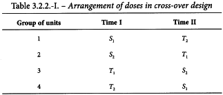
3.2.2.4. Cross-over design
This design is useful when the experiment can be sub-divided into blocks but it is possible to apply only 2 treatments to each block. For example, a block may be a single unit that can be tested on 2 occasions. The design is intended to increase precision by eliminating the effects of differences between units while balancing the effect of any difference between general levels of response at the 2 occasions. If 2 doses of a standard and of an unknown preparation are tested, this is known as a twin cross-over test.
The experiment is divided into 2 parts separated by a suitable time interval. Units are divided into 4 groups and each group receives 1 of the 4 treatments in the first part of the test. Units that received one preparation in the first part of the test receive the other preparation on the second occasion, and units receiving small doses in one part of the test receive large doses in the other. The arrangement of doses is shown in Table 3.2.2.-I. An example can be found in Section 5.1.5.
3.2.3. Analysis of variance
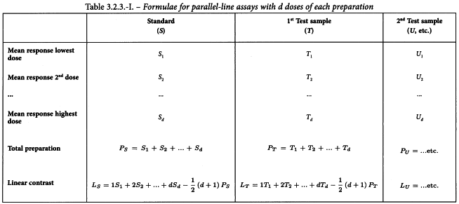
This section gives formulae that are required to carry out the analysis of variance and will be more easily understood by reference to the worked examples in Section 5.1. Reference should also be made to the glossary of symbols (Section 9).
The formulae are appropriate for symmetrical assays where one or more preparations to be examined (T, U, etc.) are compared with a standard preparation (S). It is stressed that the formulae can only be used if the doses are equally spaced, if equal numbers of treatments per preparation are applied, and each treatment is applied an equal number of times. It should not be attempted to use the formulae in any other situation.
Apart from some adjustments to the error term, the basic analysis of data derived from an assay is the same for completely randomised, randomised block and Latin square designs. The formulae for cross-over tests do not entirely fit this scheme and these are incorporated into Example 5.1.5.
Having considered the points discussed in Section 3.1 and transformed the responses, if necessary, the values should be averaged over each treatment and each preparation, as shown in Table 3.2.3.-I. The linear contrasts, which relate to the slopes of the ln(dose)-response lines, should also be formed. 3 additional formulae, which are necessary for the construction of the analysis of variance, are shown in Table 3.2.3.-II.


The total variation in response caused by the different treatments is now partitioned as shown in Table 3.2.3.-III the sums of squares being derived from the values obtained in Tables 3.2.3.-I and 3.2.3.-II. The sum of squares due to non-linearity can only be calculated if at least 3 doses per preparation are included in the assay.
The residual error of the assay is obtained by subtracting the variations allowed for in the design from the total variation in response (Table 3.2.3.-IV). In this table  represents the mean of all responses recorded in the assay. It should be noted that for a Latin square the number of replicate responses (n) is equal to the number of rows, columns or treatments (dh).
The analysis of variance is now completed as follows. Each sum of squares is divided by the corresponding number of degrees of freedom to give mean squares. The mean square for each variable to be tested is now expressed as a ratio to the residual error (s2) and the significance of these values (known as F-ratios) are assessed by use of Table 8.1 or a suitable sub-routine of a computer program.
3.2.4. Tests of validity
Assay results are said to be “statistically valid” if the outcome of the analysis of variance is as follows.
1) The linear regression term is significant, i.e. the calculated probability is less than 0.05. If this criterion is not met, it is not possible to calculate 95 per cent confidence limits.
2) The term for non-parallelism is not significant, i.e. the calculated probability is not less than 0.05. This indicates that condition 5A, Section 3.1, is satisfied.
3) The term for non-linearity is not significant, i.e. the calculated probability is not less than 0.05. This indicates that condition 4A, Section 3.1, is satisfied.
A significant deviation from parallelism in a multiple assay may be due to the inclusion in the assay-design of a preparation to be examined that gives an ln(dose)-response line with a slope different from those for the other preparations. Instead of declaring the whole assay invalid, it may then be decided to eliminate all data relating to that preparation and to restart the analysis from the beginning.
When statistical validity is established, potencies and confidence limits may be estimated by the methods described in the next section.
3.2.5. Estimation of potency and confidence limits
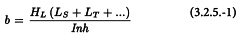
If I is the ln of the ratio between adjacent doses of any preparation, the common slope (b) for assays with d doses of each preparation is obtained from:
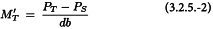
and the logarithm of the potency ratio of a test preparation, for example T, is:
The calculated potency is an estimate of the “true potency” of each unknown. Confidence limits may be calculated as the antilogarithms of:
The value of t may be obtained from Table 8.2 for p = 0.05 and degrees of freedom equal to the number of the degrees of freedom of the residual error. The estimated potency (RT) and associated confidence limits are obtained by multiplying the values obtained by AT after antilogarithms have been taken. If the stock solutions are not exactly equipotent on the basis of assigned and assumed potencies, a correction factor is necessary (See Examples 5.1.2 and 5.1.3).
3.2.6. Missing values
In a balanced assay, an accident totally unconnected with the applied treatments may lead to the loss of one or more responses, for example because an animal dies. If it is considered that the accident is in no way connected with the composition of the preparation administered, the exact calculations can still be performed but the formulae are necessarily more complicated and can only be given within the framework of general linear models (see Section 7.1). However, there exists an approximate method which keeps the simplicity of the balanced design by replacing the missing response by a calculated value. The loss of information is taken into account by diminishing the degrees of freedom for the total sum of squares and for the residual error by the number of missing values and using one of the formulae below for the missing values. It should be borne in mind that this is only an approximate method, and that the exact method is to be preferred.
If more than one observation is missing, the same formulae can be used. The procedure is to make a rough guess at all the missing values except one, and to use the proper formula for this one, using all the remaining values including the rough guesses. Fill in the calculated value. Continue by similarly calculating a value for the first rough guess. After calculating all the missing values in this way the whole cycle is repeated from the beginning, each calculation using the most recent guessed or calculated value for every response to which the formula is being applied. This continues until 2 consecutive cycles give the same values; convergence is usually rapid.
Provided that the number of values replaced is small relative to the total number of observations in the full experiment (say less than 5 per cent), the approximation implied in this replacement and reduction of degrees of freedom by the number of missing values so replaced is usually fairly satisfactory. The analysis should be interpreted with great care however, especially if there is a preponderance of missing values in one treatment or block, and a biometrician should be consulted if any unusual features are encountered. Replacing missing values in a test without replication is a particularly delicate operation.
Completely randomised design
In a completely randomised assay the missing value can be replaced by the arithmetic mean of the other responses to the same treatment.
Randomised block design
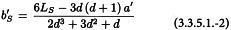
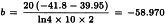
The missing value is obtained using the equation:
where B′ is the sum of the responses in the block containing the missing value, T′ the corresponding treatment total and G′ is the sum of all responses recorded in the assay.
Latin square design
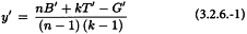
The missing value y′ is obtained from:

where B′ and C′ are the sums of the responses in the row and column containing the missing value. In this case k = n.
Cross-over design
If an accident leading to loss of values occurs in a cross-over design, a book on statistics should be consulted (e.g. D.J. Finney, see Section 10), because the appropriate formulae depend upon the particular treatment combinations.
3.3. THE SLOPE-RATIO MODEL
3.3.1. Introduction
This model is suitable, for example, for some microbiological assays when the independent variable is the concentration of an essential growth factor below the optimal concentration of the medium. The slope-ratio model is illustrated in Figure 3.3.1.-I.
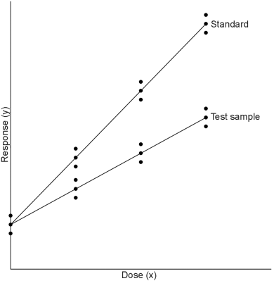
The doses are represented on the horizontal axis with zero concentration on the left and the highest concentration on the right. The responses are indicated on the vertical axis. The individual responses to each treatment are indicated with black dots. The 2 lines are the calculated dose-response relationship for the standard and the unknown under the assumption that they intersect each other at zero-dose. Unlike the parallel-line model, the doses are not transformed to logarithms.
Just as in the case of an assay based on the parallel-line model, it is important that the assumed potency is close to the true potency, and to prepare equipotent dilutions of the test preparations and the standard (if feasible). The more nearly correct the assumed potency, the closer the 2 lines will be together. The ratio of the slopes represents the “true” potency of the unknown, relative to its assumed potency. If the slope of the unknown preparation is steeper than that of the standard, the potency was underestimated and the calculations will indicate an estimated potency higher than the assumed potency. Similarly, if the slope of the unknown is less steep than that of the standard, the potency was overestimated and the calculations will result in an estimated potency lower than the assumed potency.
In setting up an experiment, all responses should be examined for the fulfilment of the conditions 1, 2 and 3 in Section 3.1. The analysis of variance to be performed in routine is described in Section 3.3.3 so that compliance with conditions 4B and 5B of Section 3.1 may be examined.
3.3.2. Assay design
The use of the statistical analysis presented below imposes the following restrictions on the assay:
a) the standard and the test preparations must be tested with the same number of equally spaced dilutions,
b) an extra group of experimental units receiving no treatment may be tested (the blanks),
c) there must be an equal number of experimental units to each treatment.
As already remarked in Section 3.1.3, assay designs not meeting these restrictions may be both possible and correct, but the simple statistical analyses presented here are no longer applicable and either expert advice should be sought or suitable software should be used.
A design with 2 doses per preparation and 1 blank, the “common zero (2h + 1)-design”, is usually preferred, since it gives the highest precision combined with the possibility to check validity within the constraints mentioned above. However, a linear relationship cannot always be assumed to be valid down to zero-dose. With a slight loss of precision a design without blanks may be adopted. In this case 3 doses per preparation, the “common zero (3h)-design”, are preferred to 2 doses per preparation. The doses are thus given as follows:
1) the standard is given in a high dose, near to but not exceeding the highest dose giving a mean response on the straight portion of the dose-response line,
2) the other doses are uniformly spaced between the highest dose and zero dose,
3) the test preparations are given in corresponding doses based on the assumed potency of the material.
A completely randomised, a randomised block or a Latin square design may be used, such as described in Section 3.2.2. The use of any of these designs necessitates an adjustment to the error sum of squares as described for assays based on the parallel-line model. The analysis of an assay of one or more test preparations against a standard is described below.
3.3.3. Analysis of variance
3.3.3.1. The (hd + 1)-design
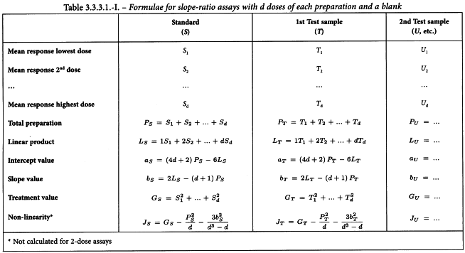
The responses are verified as described in Section 3.1 and, if necessary, transformed. The responses are then averaged over each treatment and each preparation as shown in Table 3.3.3.1.-I. Additionally, the mean response for blanks (B) is calculated.
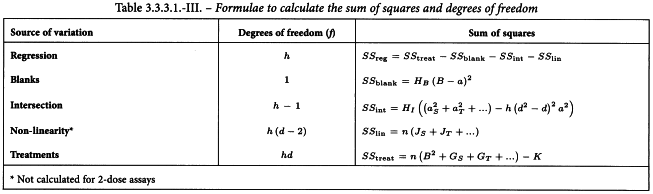
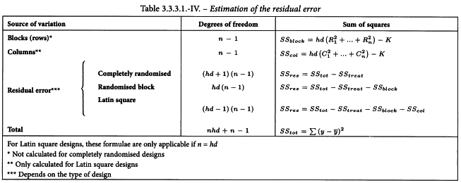
The sums of squares in the analysis of variance are calculated as shown in Tables 3.3.3.1.-I to 3.3.3.1.-III. The sum of squares due to non-linearity can only be calculated if at least 3 doses of each preparation have been included in the assay. The residual error is obtained by subtracting the variations allowed for in the design from the total variation in response (Table 3.3.3.1.-IV).

The analysis of variance is now completed as follows. Each sum of squares is divided by the corresponding number of degrees of freedom to give mean squares. The mean square for each variable to be tested is now expressed as a ratio to the residual error (s2) and the significance of these values (known as F-ratios) are assessed by use of Table 8.1 or a suitable sub-routine of a computer program.
3.3.3.2. The (hd)-design
The formulae are basically the same as those for the (hd + 1)-design, but there are some slight differences.
Validity of the assay, potency and confidence interval are found as described in Sections 3.3.4 and 3.3.5.
3.3.4. Tests of validity
Assay results are said to be “statistically valid” if the outcome of the analysis of variance is as follows:
1) the variation due to blanks in (hd + 1)-designs is not significant, i.e. the calculated probability is not smaller than 0.05. This indicates that the responses of the blanks do not significantly differ from the common intercept and the linear relationship is valid down to zero dose;
2) the variation due to intersection is not significant, i.e. the calculated probability is not less than 0.05. This indicates that condition 5B, Section 3.1 is satisfied;
3) in assays including at least 3 doses per preparation, the variation due to non-linearity is not significant, i.e. the calculated probability is not less than 0.05. This indicates that condition 4B, Section 3.1 is satisfied.
A significant variation due to blanks indicates that the hypothesis of linearity is not valid near zero dose. If this is likely to be systematic rather than incidental for the type of assay, the (hd-design) is more appropriate. Any response to blanks should then be disregarded.
When these tests indicate that the assay is valid, the potency is calculated with its confidence limits as described in Section 3.3.5.
3.3.5. Estimation of potency and confidence limits
3.3.5.1. The (hd + 1)-design
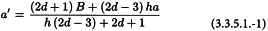
The common intersection a′ of the preparations can be calculated from:
The slope of the standard, and similarly for each of the other preparations, is calculated from:
The potency ratio of each of the test preparations can now be calculated from:
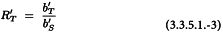
which has to be multiplied by AT, the assumed potency of the test preparation, in order to find the estimated potency RT. If the step between adjacent doses was not identical for the standard and the test preparation, the potency has to be multiplied by IS/IT. Note that, unlike the parallel-line analysis, no antilogarithms are calculated.
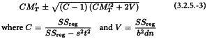
The confidence interval for RT′ is calculated from:
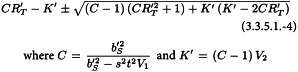
V1 and V2 are related to the variance and covariance of the numerator and denominator of RT. They can be obtained from:
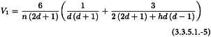
The confidence limits are multiplied by AT, and if necessary by IS/IT.
3.3.5.2. The (hd)-design
The formulae are the same as for the (hd + 1)-design, with the following modifications:

3.4. EXTENDED SIGMOID DOSE-RESPONSE CURVES
This model is suitable, for example, for some immunoassays when analysis is required of extended sigmoid dose-response curves. This model is illustrated in Figure 3.4.-I.
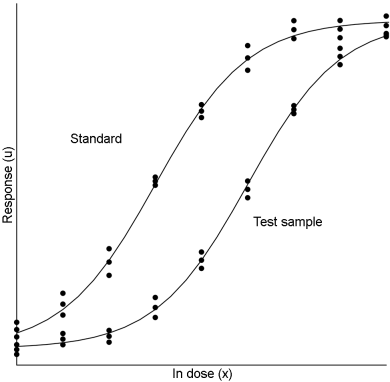
The logarithms of the doses are represented on the horizontal axis with the lowest concentration on the left and the highest concentration on the right. The responses are indicated on the vertical axis. The individual responses to each treatment are indicated with black dots. The 2 curves are the calculated ln(dose)-response relationship for the standard and the test preparation.
The general shape of the curves can usually be described by a logistic function but other shapes are also possible. Each curve can be characterised by 4 parameters: The upper asymptote (α), the lower asymptote (δ), the slope-factor (β), and the horizontal location (γ). This model is therefore often referred to as a four-parameter model. A mathematical representation of the ln(dose)-response curve is:
For a valid assay it is necessary that the curves of the standard and the test preparations have the same slope-factor, and the same maximum and minimum response level at the extreme parts. Only the horizontal location (γ) of the curves may be different. The horizontal distance between the curves is related to the “true” potency of the unknown. If the assay is used routinely, it may be sufficient to test the condition of equal upper and lower response levels when the assay is developed, and then to retest this condition directly only at suitable intervals or when there are changes in materials or assay conditions.
The maximum-likelihood estimates of the parameters and their confidence intervals can be obtained with suitable computer programs. These computer programs may include some statistical tests reflecting validity. For example, if the maximum likelihood estimation shows significant deviations from the fitted model under the assumed conditions of equal upper and lower asymptotes and slopes, then one or all of these conditions may not be satisfied.
The logistic model raises a number of statistical problems which may require different solutions for different types of assays, and no simple summary is possible. A wide variety of possible approaches is described in the relevant literature. Professional advice is therefore recommended for this type of analysis. A simple example is nevertheless included in Section 5.4 to illustrate a “possible” way to analyse the data presented. A short discussion of alternative approaches and other statistical considerations is given in Section 7.5.
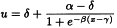
If professional advice or suitable software is not available, alternative approaches are possible: 1) if “reasonable” estimates of the upper limit (α) and lower limit (δ) are available, select for all preparations the doses with mean of the responses (u) falling between approximately 20 per cent and 80 per cent of the limits, transform responses of the selected doses to:

and use the parallel line model (Section 3.2) for the analysis; 2) select a range of doses for which the responses (u) or suitably transformed responses, for example ln u, are approximately linear when plotted against ln(dose); the parallel line model (Section 3.2) may then be used for analysis.
4. Assays depending upon quantal responses
4.1. INTRODUCTION
In certain assays it is impossible or excessively laborious to measure the effect on each experimental unit on a quantitative scale. Instead, an effect such as death or hypoglycaemic symptoms may be observed as either occurring or not occurring in each unit, and the result depends on the number of units in which it occurs. Such assays are called quantal or all-or-none.
The situation is very similar to that described for quantitative assays in Section 3.1, but in place of n separate responses to each treatment a single value is recorded, i.e. the fraction of units in each treatment group showing a response. When these fractions are plotted against the logarithms of the doses the resulting curve will tend to be sigmoid (S-shaped) rather than linear. A mathematical function that represents this sigmoid curvature is used to estimate the dose-response curve. The most commonly used function is the cumulative normal distribution function. This function has some theoretical merit, and is perhaps the best choice if the response is a reflection of the tolerance of the units. If the response is more likely to depend upon a process of growth, the logistic distribution model is preferred, although the difference in outcome between the 2 models is usually very small.
The maximum likelihood estimators of the slope and location of the curves can be found only by applying an iterative procedure. There are many procedures which lead to the same outcome, but they differ in efficiency due to the speed of convergence. One of the most rapid methods is direct optimisation of the maximum-likelihood function (see Section 7.1), which can easily be performed with computer programs having a built-in procedure for this purpose. Unfortunately, most of these procedures do not yield an estimate of the confidence interval, and the technique to obtain it is too complicated to describe here. The technique described below is not the most rapid, but has been chosen for its simplicity compared to the alternatives. It can be used for assays in which one or more test preparations are compared to a standard. Furthermore, the following conditions must be fulfilled:
1) the relationship between the logarithm of the dose and the response can be represented by a cumulative normal distribution curve,
2) the curves for the standard and the test preparation are parallel, i.e. they are identically shaped and may only differ in their horizontal location,
3) in theory, there is no natural response to extremely low doses and no natural non-response to extremely high doses.
4.2. THE PROBIT METHOD
The sigmoid curve can be made linear by replacing each response, i.e. the fraction of positive responses per group, by the corresponding value of the cumulative standard normal distribution. This value, often referred to as “normit”, ranges theoretically from -∞ to + ∞. In the past it was proposed to add 5 to each normit to obtain “probits”. This facilitated the hand-performed calculations because negative values were avoided. With the arrival of computers the need to add 5 to the normits has disappeared. The term “normit method” would therefore be better for the method described below. However, since the term “probit analysis” is so widely spread, the term will, for historical reasons, be maintained in this text.
Once the responses have been linearised, it should be possible to apply the parallel-line analysis as described in Section 3.2. Unfortunately, the validity condition of homogeneity of variance for each dose is not fulfilled. The variance is minimal at normit = 0 and increases for positive and negative values of the normit. It is therefore necessary to give more weight to responses in the middle part of the curve, and less weight to the more extreme parts of the curve. This method, the analysis of variance, and the estimation of the potency and confidence interval are described below.
4.2.1. Tabulation of the results
Table 4.2.1.-I is used to enter the data into the columns indicated by numbers:
(1) the dose of the standard or the test preparation,
(2) the number n of units submitted to that treatment,
(3) the number of units R giving a positive response to the treatment,
(4) the logarithm x of the dose,
(5) the fraction p = r/n of positive responses per group.
The first cycle starts here.
(6) column Y is filled with zeros at the first iteration,
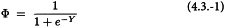
(7) the corresponding value Φ = Φ(Y) of the cumulative standard normal distribution function (see also Table 8.4).
The columns (8) to (10) are calculated with the following formulae:


The columns (11) to (15) can easily be calculated from columns (4), (9) and (10) as wx, wy, wx2, wy2 and wxy respectively, and the sum (Σ) of each of the columns (10) to (15) is calculated separately for each of the preparations.

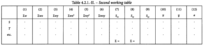
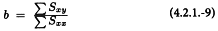
The sums calculated in Table 4.2.1.-I are transferred to columns (1) to (6) of Table 4.2.1.-II and 6 additional columns (7) to (12) are calculated as follows:


The common slope b can now be obtained as:
and the intercept a of the standard, and similarly for the test preparations is obtained as:

Column (6) of the first working table can now be replaced by Y = a + bx and the cycle is repeated until the difference between 2 cycles has become small (e.g. the maximum difference of Y between 2 consecutive cycles is smaller than 10-8).
4.2.2. Tests of validity
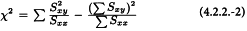
Before calculating the potencies and confidence intervals, validity of the assay must be assessed. If at least 3 doses for each preparation have been included, the deviations from linearity can be measured as follows: add a 13th column to Table 4.2.1.-II and fill it with:
The column total is a measure of deviations from linearity and is approximately χ2 distributed with degrees of freedom equal to N -2h. Significance of this value may be assessed with the aid of Table 8.3 or a suitable sub-routine in a computer program. If the value is significant at the 0.05 probability level, the assay must probably be rejected (see Section 4.2.4).
When the above test gives no indication of significant deviations from linear regression, the deviations from parallelism are tested at the 0.05 significance level with:
with h- 1 degrees of freedom.
4.2.3. Estimation of potency and confidence limits
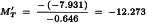
When there are no indications for a significant departure from parallelism and linearity the ln(potency ratio) M′T is calculated as:
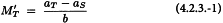
and the antilogarithm is taken. Now let t = 1.96 and s = 1. Confidence limits are calculated as the antilogarithms of:
4.2.4. Invalid assays
If the test for deviations from linearity described in Section 4.2.2 is significant, the assay should normally be rejected. If there are reasons to retain the assay, the formulae are slightly modified. t becomes the t-value (p = 0.05) with the same number of degrees of freedom as used in the check for linearity and s2 becomes the χ2 value divided by the same number of degrees of freedom (and thus typically is greater than 1).
The test for parallelism is also slightly modified. The χ2 value for non-parallelism is divided by its number of degrees of freedom. The resulting value is divided by s2 calculated above to obtain an F-ratio with h - 1 and N - 2h degrees of freedom, which is evaluated in the usual way at the 0.05 significance level.
4.3. THE LOGIT METHOD
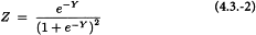
As indicated in Section 4.1 the logit method may sometimes be more appropriate. The name of the method is derived from the logit function which is the inverse of the logistic distribution. The procedure is similar to that described for the probit method with the following modifications in the formulae for Φ and Z.
4.4. OTHER SHAPES OF THE CURVE
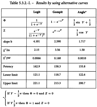
The probit and logit method are almost always adequate for the analysis of quantal responses called for in the European Pharmacopoeia. However, if it can be made evident that the ln(dose)-response curve has another shape than the 2 curves described above, another curve Φ may be adopted. Z is then taken to be the first derivative of Φ.
For example, if it can be shown that the curve is not symmetric, the Gompertz distribution may be appropriate (the gompit method) in which case  and
and  .
.
4.5. THE MEDIAN EFFECTIVE DOSE
In some types of assay it is desirable to determine a median effective dose which is the dose that produces a response in 50 per cent of the units. The probit method can be used to determine this median effective dose (ED50), but since there is no need to express this dose relative to a standard, the formulae are slightly different.
Note A standard can optionally be included in order to validate the assay. Usually the assay is considered valid if the calculated ED50 of the standard is close enough to the assigned ED50. What “close enough” in this context means depends on the requirements specified in the monograph.
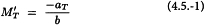
The tabulation of the responses to the test samples, and optionally a standard, is as described in Section 4.2.1. The test for linearity is as described in Section 4.2.2. A test for parallelism is not necessary for this type of assay. The ED50 of test sample T, and similarly for the other samples, is obtained as described in Section 4.2.3, with the following modifications in formulae 4.2.3.-1 and 4.2.3.-2:
5. Examples
This section consists of worked examples illustrating the application of the formulae. The examples have been selected primarily to illustrate the statistical method of calculation. They are not intended to reflect the most suitable method of assay, if alternatives are permitted in the individual monographs. To increase their value as program checks, more decimal places are given than would usually be necessary. It should also be noted that other, but equivalent methods of calculation exist. These methods should lead to exactly the same final results as those given in the examples.
5.1. PARALLEL-LINE MODEL
5.1.1. Two-dose multiple assay with completely randomised design
An assay of corticotrophin by subcutaneous injection in rats
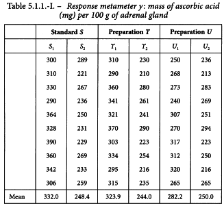
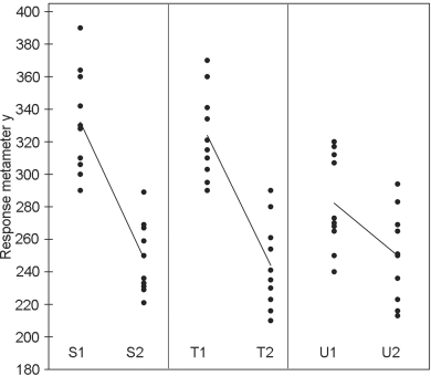
The standard preparation is administered at 0.25 and 1.0 units per 100 g of body mass. Two preparations to be examined are both assumed to have a potency of 1 unit per milligram and they are administered in the same quantities as the standard. The individual responses and means per treatment are given in Table 5.1.1.-I. A graphical presentation (Figure 5.1.1.-I) gives no rise to doubt the homogeneity of variance and normality of the data, but suggests problems with parallelism for preparation U.
The formulae in Tables 3.2.3.-I and 3.2.3.-II lead to:
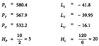
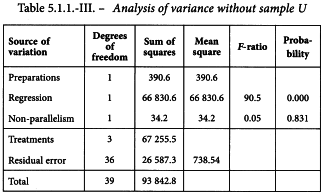
The analysis of variance can now be completed with the formulae in Tables 3.2.3-III and 3.2.3.-IV. This is shown in Table 5.1.1.-II.
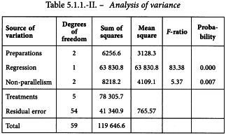
The analysis confirms a highly significant linear regression. Departure from parallelism, however, is also significant (p = 0.0075) which was to be expected from the graphical observation that preparation U is not parallel to the standard. This preparation is therefore rejected and the analysis repeated using only preparation T and the standard (Table 5.1.1.-III).
The analysis without preparation U results in compliance with the requirements with respect to both regression and parallelism and so the potency can be calculated. The formulae in Section 3.2.5 give:
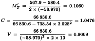
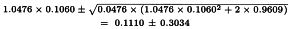
By taking the antilogarithms we find a potency ratio of 1.11 with 95 per cent confidence limits from 0.82-1.51.
Multiplying by the assumed potency of preparation T yields a potency of 1.11 units/mg with 95 per cent confidence limits from 0.82 to 1.51 units/mg.
5.1.2. Three-dose Latin square design
Antibiotic agar diffusion assay using a rectangular tray
The standard has an assigned potency of 4855 IU/mg. The test preparation has an assumed potency of 5600 IU/mg. For the stock solutions 25.2 mg of the standard is dissolved in 24.5 mL of solvent and 21.4 mg of the test preparation is dissolved in 23.95 mL of solvent. The final solutions are prepared by first diluting both stock solutions to 1/20 and further using a dilution ratio of 1.5.
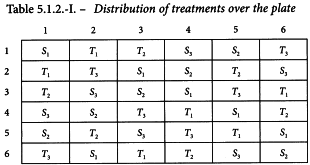
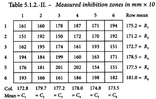
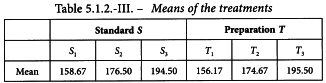
A Latin square is generated with the method described in Section 8.6 (see Table 5.1.2.-I). The responses of this routine assay are shown in Table 5.1.2.-II (inhibition zones in mm × 10). The treatment mean values are shown in Table 5.1.2.-III. A graphical representation of the data (see Figure 5.1.2.-I) gives no rise to doubt the normality or homogeneity of variance of the data.
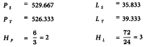
The formulae in Tables 3.2.3.-I and 3.2.3.-II lead to:
The analysis of variance can now be completed with the formulae in Tables 3.2.3.-III and 3.2.3.-IV. The result is shown in Table 5.1.2.-IV.
The analysis shows significant differences between the rows. This indicates the increased precision achieved by using a Latin square design rather than a completely randomised design. A highly significant regression and no significant departure of the individual regression lines from parallelism and linearity confirms that the assay is satisfactory for potency calculations.


The formulae in Section 3.2.5 give:


The potency ratio is found by taking the antilogarithms, resulting in 0.9763 with 95 per cent confidence limits from 0.9112-1.0456.
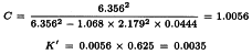
A correction factor of:
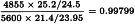
is necessary because the dilutions were not exactly equipotent on the basis of the assumed potency. Multiplying by this correction factor and the assumed potency of 5600 IU/mg yields a potency of 5456 IU/mg with 95 per cent confidence limits from 5092 to 5843 IU/mg.
5.1.3. Four-dose randomised block design
Antibiotic turbidimetric assay
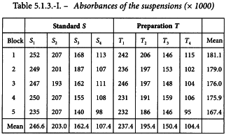
This assay is designed to assign a potency in international units per vial. The standard has an assigned potency of 670 IU/mg. The test preparation has an assumed potency of 20 000 IU/vial. On the basis of this information the stock solutions are prepared as follows. 16.7 mg of the standard is dissolved in 25 mL solvent and the contents of one vial of the test preparation are dissolved in 40 mL solvent. The final solutions are prepared by first diluting to 1/40 and further using a dilution ratio of 1.5. The tubes are placed in a water-bath in a randomised block arrangement (see Section 8.5). The responses are listed in Table 5.1.3.-I.
Inspection of Figure 5.1.3.-I gives no rise to doubt the validity of the assumptions of normality and homogeneity of variance of the data. The standard deviation of S3 is somewhat high but is no reason for concern.

The formulae in Tables 3.2.3.-I and 3.2.3.-II lead to:
The analysis of variance is constructed with the formulae in Tables 3.2.3.-III and 3.2.3.-IV. The result is shown in Table 5.1.3.-II.
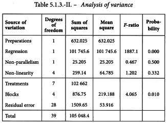
A significant difference is found between the blocks. This indicates the increased precision achieved by using a randomised block design. A highly significant regression and no significant departure from parallelism and linearity confirms that the assay is satisfactory for potency calculations. The formulae in Section 3.2.5 give:
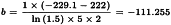
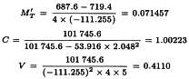
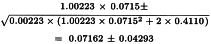
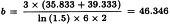
The potency ratio is found by taking the antilogarithms, resulting in 1.0741 with 95 per cent confidence limits from 1.0291 to 1.1214. A correction factor of:
is necessary because the dilutions were not exactly equipotent on the basis of the assumed potency. Multiplying by this correction factor and the assumed potency of 20 000 IU/vial yields a potency of 19 228 IU/vial with 95 per cent confidence limits from 18 423-20 075 IU/vial.
5.1.4. Five-dose multiple assay with completely randomised design
An in-vitro assay of three hepatitis B vaccines against a standard
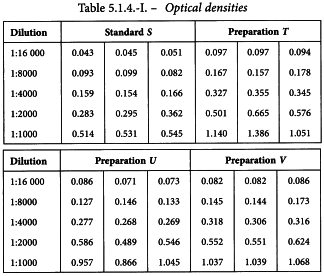
Three independent two-fold dilution series of 5 dilutions were prepared from each of the vaccines. After some additional steps in the assay procedure, absorbances were measured. They are shown in Table 5.1.4.-I.
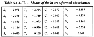
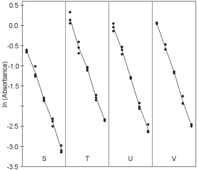
The logarithms of the optical densities are known to have a linear relationship with the logarithms of the doses. The mean responses of the ln-transformed optical densities are listed in Table 5.1.4.-II. No unusual features are discovered in a graphical presentation of the data (Figure 5.1.4.-I).
The formulae in Tables 3.2.3.-I and 3.2.3.-II give:
The analysis of variance is completed with the formulae in Tables 3.2.3.-III and 3.2.3.-IV. This is shown in Table 5.1.4.-III.

A highly significant regression and a non-significant departure from parallelism and linearity confirm that the potencies can be safely calculated. The formulae in Section 3.2.5 give:
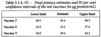
By taking the antilogarithms a potency ratio of 2.171 is found with 95 per cent confidence limits from 2.027 to 2.327. All samples have an assigned potency of 20 µg protein/mL and so a potency of 43.4 µg protein/mL is found for test preparation T with 95 per cent confidence limits from 40.5-46.5 µg protein/mL.
The same procedure is followed to estimate the potency and confidence interval of the other test preparations. The results are listed in Table 5.1.4.-IV.
5.1.5. Twin cross-over design
Assay of insulin by subcutaneous injection in rabbits
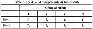
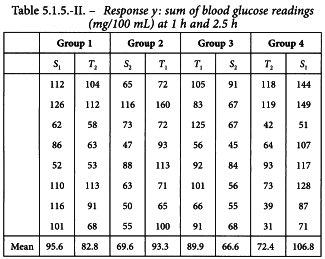
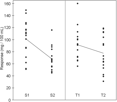
The standard preparation was administered at 1 unit and 2 units per millilitre. Equivalent doses of the unknown preparation were used based on an assumed potency of 40 units per millilitre. The rabbits received subcutaneously 0.5 mL of the appropriate solutions according to the design in Table 5.1.5.-I and responses obtained are shown in Table 5.1.5.-II and Figure 5.1.5.-I. The large variance illustrates the variation between rabbits and the need to employ a cross-over design.
The analysis of variance is more complicated for this assay than for the other designs given because the component of the sum of squares due to parallelism is not independent of the component due to rabbit differences. Testing of the parallelism of the regression lines involves a second error-mean-square term obtained by subtracting the parallelism component and 2 “interaction” components from the component due to rabbit differences.
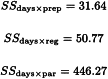
Three “interaction” components are present in the analysis of variance due to replication within each group:
days × preparation; days × regression; days × parallelism.
These terms indicate the tendency for the components (preparations, regression and parallelism) to vary from day to day. The corresponding F-ratios thus provide checks on these aspects of assay validity. If the values of F obtained are significantly high, care should be exercised in interpreting the results of the assay and, if possible, the assay should be repeated.
The analysis of variance is constructed by applying the formulae given in Tables 3.2.3.-I to 3.2.3.-III separately for both days and for the pooled set of data. The formulae in Tables 3.2.3.-I and 3.2.3.-II give:
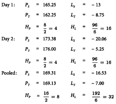
and with the formulae in Table 3.2.3.-III this leads to:
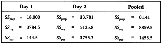
The interaction terms are found as Day 1 + Day 2 - Pooled.
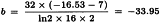
In addition the sum of squares due to day-to-day variation is calculated as:

and the sum of squares due to blocks (the variation between rabbits) as:
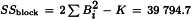
where Bi is the mean response per rabbit.
The analysis of variance can now be completed as shown in Table 5.1.5.-III.
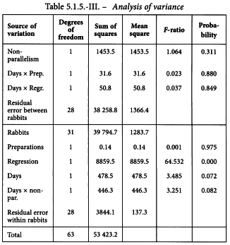
The analysis of variance confirms that the data fulfil the necessary conditions for a satisfactory assay: a highly significant regression, no significant departures from parallelism, and none of the three interaction components is significant.
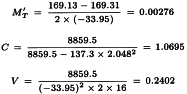
The formulae in Section 3.2.5 give:
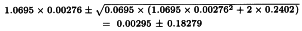
By taking the antilogarithms a potency ratio of 1.003 with 95 per cent confidence limits from 0.835 to 1.204 is found. Multiplying by AT = 40 yields a potency of 40.1 units per millilitre with 95 per cent confidence limits from 33.4-48.2 units per millilitre.
5.2. SLOPE-RATIO MODEL
5.2.1. A completely randomised (0,3,3)-design
An assay of factor VIII
A laboratory carries out a chromogenic assay of factor VIII activity in concentrates. The laboratory has no experience with the type of assay but is trying to make it operational. Three equivalent dilutions are prepared of both the standard and the test preparation. In addition a blank is prepared, although a linear dose-response relationship is not expected for low doses. 8 replicates of each dilution are prepared, which is more than would be done in a routine assay.
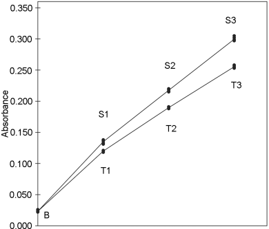
A graphical presentation of the data shows clearly that the dose-response relationship is indeed not linear at low doses. The responses to blanks will therefore not be used in the calculations (further assays are of course needed to justify this decision). The formulae in Tables 3.3.3.1.-I and 3.3.3.1.-II yield:
and

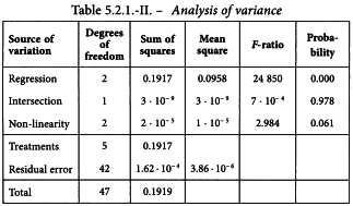
and the analysis of variance is completed with the formulae in Tables 3.3.3.1.-III and 3.3.3.1.-IV.
A highly significant regression and no significant deviations from linearity and intersection indicate that the potency can be calculated.
Slope of standard:
Slope of test sample:
Formula 3.3.5.1.-3 gives:
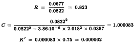
and the 95 per cent confidence limits are:
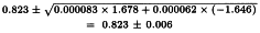
The potency ratio is thus estimated as 0.823 with 95 per cent confidence limits from 0.817 to 0.829.
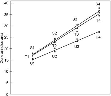
5.2.2. A completely randomised (0,4,4,4)-design
An in-vitro assay of influenza vaccines
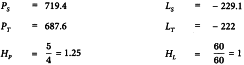
The haemagglutinin antigen (HA) content of 2 influenza vaccines is determined by single radial immunodiffusion. Both have a labelled potency of 15 µg HA per dose, which is equivalent with a content of 30 µg HA/mL. The standard has an assigned content of 39 µg HA/mL.
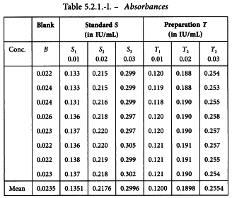
Standard and test vaccines are applied in 4 duplicate concentrations which are prepared on the basis of the assigned and the labelled contents. When the equilibrium between the external and the internal reactant is established, the zone of the annulus precipitation area is measured. The results are shown in Table 5.2.2.-I.
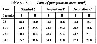
A graphical presentation of the data shows no unusual features (see Figure 5.2.2.-I). The formulae in Tables 3.3.3.1.-I and 3.3.3.1.-II yield:
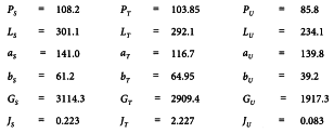
and

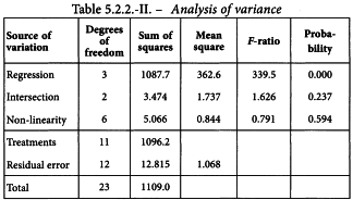
and the analysis of variance is completed with the formulae in Tables 3.3.3.1.-III and 3.3.3.1.-IV. This is shown in Table 5.2.2.-II.
A highly significant regression and no significant deviations from linearity and intersection indicate that the potency can be calculated.
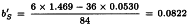
Slope of standard:
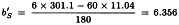
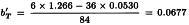
Slope of T is:
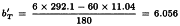
Slope of U is:

This leads to a potency ratio of 6.056/6.356 = 0.953 for vaccine T and 4.123/6.356 = 0.649 for vaccine U.
And the confidence limits are found with formula 3.3.5.1.-4.
For vaccine T:

For vaccine U:

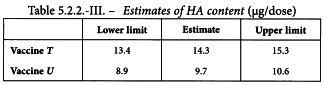
The HA content in µg/dose can be found by multiplying the potency ratios and confidence limits by the assumed content of 15 µg/dose. The results are given in Table 5.2.2.-III.
5.3. QUANTAL RESPONSES
5.3.1. Probit analysis of a test preparation against a reference
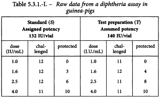
An in-vivo assay of a diphtheria vaccine
A diphtheria vaccine (assumed potency 140 IU/vial) is assayed against a standard (assigned potency 132 IU/vial). On the basis of this information, equivalent doses are prepared and randomly administered to groups of guinea-pigs. After a given period, the animals are challenged with diphtheria toxin and the number of surviving animals recorded as shown in Table 5.3.1.-I.
The observations are transferred to the first working table and the subsequent columns are computed as described in Section 4.2.1. Table 5.3.1.-II shows the first cycle of this procedure.
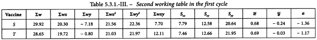
The sums of the last 6 columns are then calculated per preparation and transferred to the second working table (see Table 5.3.1.-III). The results in the other columns are found with formulae 4.2.1.-4 to 4.2.1.-10. This yields a common slope b of 1.655.
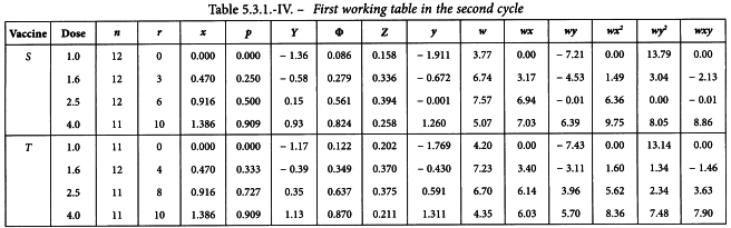
The values for Y in the first working table are now replaced by a + bx and a second cycle is carried out (see Table 5.3.1.-IV).
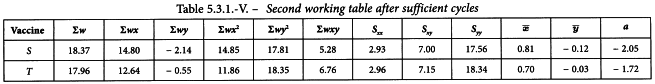
The cycle is repeated until the difference between 2 consecutive cycles has become small. The second working table should then appear as shown in Table 5.3.1.-V.

Linearity is tested as described in Section 4.2.2. The χ2-value with 4 degrees of freedom is 0.851 + 1.070 = 1.921 representing a p-value of 0.750 which is not significant.
Since there are no significant deviations from linearity, the test for parallelism can be carried out as described in the same section. The χ2-value with 1 degree of freedom is:
representing a p-value of 0.974 which is not significant.
The ln(potency ratio) can now be estimated as described in Section 4.2.3.
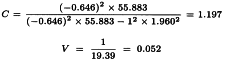
Further:
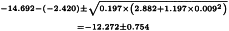
So ln confidence limits are:

The potency and confidence limits can now be found by taking the antilogarithms and multiplying these by the assumed potency of 140 IU/vial. This yields an estimate of 160.6 IU/vial with 95 per cent confidence limits from 121.0-215.2 IU/vial.
5.3.2. Logit analysis and other types of analyses of a test preparation against a reference
Results will be given for the situation where the logit method and other “classical” methods of this family are applied to the data in Section 5.3.1. This should be regarded as an exercise rather than an alternative to the probit method in this specific case. Another shape of the curve may be adopted only if this is supported by experimental or theoretical evidence. See Table 5.3.2.-I.
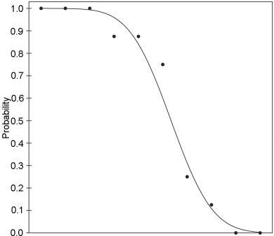
5.3.3. The ED50 determination of a substance using the probit method
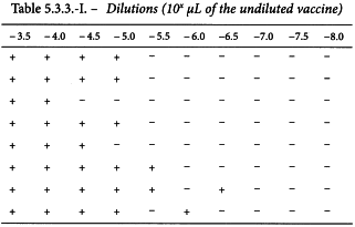
An in-vitro assay of oral poliomyelitis vaccine
In an ED50 assay of oral poliomyelitis vaccine with 10 different dilutions in 8 replicates of 50 µL on an ELISA-plate, results were obtained as shown in Table 5.3.3.-I.
The observations are transferred to the first working table and the subsequent columns are computed as described in Section 4.2.1. Table 5.3.3.-II shows the first cycle of this procedure.
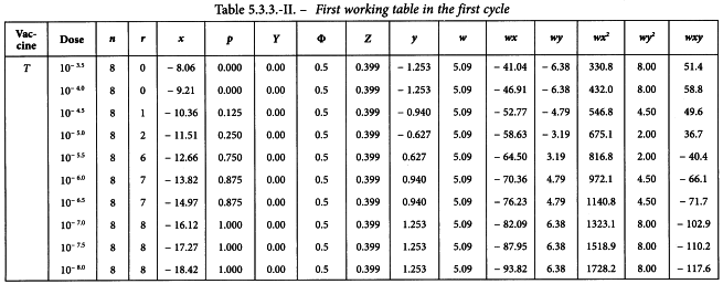
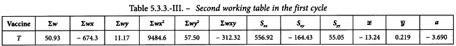
The sums of the last 6 columns are calculated and transferred to the second working table (see Table 5.3.3.-III). The results in the other columns are found with formulae 4.2.1.-4 to 4.2.1.-10. This yields a common slope b of -0.295.
The values for Y in the first working table are now replaced by a + bx and a second cycle is carried out. The cycle is repeated until the difference between 2 consecutive cycles has become small. The second working table should then appear as shown in Table 5.3.3.-IV.

Linearity is tested as described in Section 4.2.2. The χ2-value with 8 degrees of freedom is 2.711 representing a p-value of 0.951 which is not significant.
The potency ratio can now be estimated as described in Section 4.5.
Further:
So ln confidence limits are:
This estimate is still expressed in terms of the ln(dilutions). In order to obtain estimates expressed in ln(ED50)/mL the values are transformed to:

Since it has become common use to express the potency of this type of vaccine in terms of log10(ED50)/mL, the results have to be divided by ln(10). The potency is thus estimated as 6.63 log10(ED50)/mL with 95 per cent confidence limits from 6.30 to 6.96 log10(ED50)/mL.
5.4. EXTENDED SIGMOID DOSE-RESPONSE CURVES
5.4.1. Four-parameter logistic curve analysis
A serological assay of tetanus sera
As already stated in Section 3.4, this example is intended to illustrate a “possible” way to analyse the data presented, but not necessarily to reflect the “only” or the “most appropriate” way. Many other approaches can be found in the literature, but in most cases they should not yield dramatically different outcomes. A short discussion of alternative approaches and other statistical considerations is given in Section 7.5.
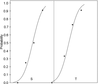
A guinea-pig antiserum is assayed against a standard serum (0.4 IU/mL) using an enzyme-linked immunosorbent assay technique (ELISA). 10 two-fold dilutions of each serum were applied on a 96-well ELISA plate. Each dilution was applied twice. The observed responses are listed in Table 5.4.1.-I.

For this example, it will be assumed that the laboratory has validated conditions 1 to 3 in Section 3.1.1 when the assay was being developed for routine use. In addition, the laboratory has validated that the upper limit and lower limit of the samples can be assumed to be equal.
No unusual features are discovered in a graphical representation. A least squares method of a suitable computer program is used to fit the parameters of the logistic function, assuming that the residual error terms are independent and identically distributed normal random variables. In this case, 3 parameters (α, β and δ) are needed to describe the common slope-factor and the common lower and upper asymptotes. 2 additional parameters (γS and γT) are needed to describe the horizontal location of the 2 curves.
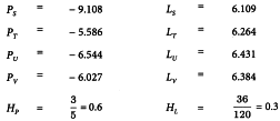
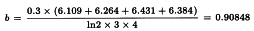
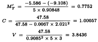
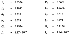
The following estimates of the parameters are returned by the program:
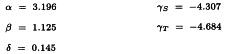
In addition, the estimated residual variance (s2) is returned as 0.001429 with 20 degrees of freedom (within-treatments variation).
In order to obtain confidence limits, and also to check for parallelism and linearity, the observed responses (u) are linearised and submitted to a weighted parallel-line analysis by the program. This procedure is very similar to that described in Section 4.2 for probit analysis with the following modifications:
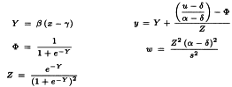
The resulting weighted analysis of variance of the transformed responses (y) using weights (w) is shown in Table 5.4.1.-II.
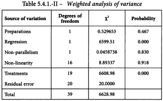
There are no significant deviations from parallelism and linearity and thus the assay is satisfactory for potency calculations. If the condition of equal upper and lower asymptotes is not fulfilled, significant deviations from linearity and/or parallelism are likely to occur because the tests for linearity and parallelism reflect the goodness of fit of the complete four-parameter model. The residual error in the analysis of variance is always equal to 1 as a result of the transformation. However, a heterogeneity factor (analogous to that for the probit model) can be computed.
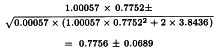
The relative potency of the test preparation can be obtained as the antilogarithm of γS-γT. Multiplying by the assigned potency of the standard yields an estimate of 1.459 × 0.4 = 0.584 IU/mL. Formula 4.2.3.-2 gives 95 per cent confidence limits from 0.557-0.612 IU/mL.
6. Combination of assay results
6.1. INTRODUCTION
Replication of independent assays and combination of their results is often needed to fulfil the requirements of the European Pharmacopoeia. The question then arises as to whether it is appropriate to combine the results of such assays and if so in what way.
Two assays may be regarded as mutually independent when the execution of either does not affect the probabilities of the possible outcomes of the other. This implies that the random errors in all essential factors influencing the result (for example, dilutions of the standard and of the preparation to be examined, the sensitivity of the biological indicator) in 1 assay must be independent of the corresponding random errors in the other one. Assays on successive days using the original and retained dilutions of the standard therefore are not independent assays.
There are several methods for combining the results of independent assays, the most theoretically acceptable being the most difficult to apply. 3 simple, approximate methods are described below; others may be used provided the necessary conditions are fulfilled.
Before potencies from assays based on the parallel-line or probit model are combined they must be expressed in logarithms; potencies derived from assays based on the slope-ratio model are used as such. As the former models are more common than those based on the slope-ratio model, the symbol M denoting ln potency is used in the formulae in this section; by reading R (slope-ratio) for M, the analyst may use the same formulae for potencies derived from assays based on the slope-ratio model. All estimates of potency must be corrected for the potency assigned to each preparation to be examined before they are combined.
6.2. WEIGHTED COMBINATION OF ASSAY RESULTS
This method can be used provided the following conditions are fulfilled:
1) the potency estimates are derived from independent assays;
2) for each assay C is close to 1 (say less than 1.1);
3) the number of degrees of freedom of the individual residual errors is not smaller than 6, but preferably larger than 15;
4) the individual potency estimates form a homogeneous set (see Section 6.2.2).
When these conditions are not fulfilled this method cannot be applied. The method described in Section 6.3 may then be used to obtain the best estimate of the mean potency to be adopted in further assays as an assumed potency.
6.2.1. Calculation of weighting coefficients
It is assumed that the results of each of the n′ assays have been analysed to give n′ values of M with associated confidence limits. For each assay the logarithmic confidence interval L is obtained by subtracting the lower limit from the upper. A weight W for each value of M is calculated from equation 6.2.1.-1, where t has the same value as that used in the calculation of confidence limits.
6.2.2. Homogeneity of potency estimates
By squaring the deviation of each value of M from the weighted mean, multiplying by the appropriate weight and summing over all assays, a statistic is obtained which is approximately distributed as χ2 (see Table 8.3) and which may be used to test the homogeneity of a set of ln potency estimates:
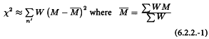
If the calculated χ2 is smaller than the tabulated value corresponding to (n′- 1) degrees of freedom the potencies are homogeneous and the mean potency and limits obtained in Section 6.2.3 will be meaningful.
If the calculated value of this statistic is greater than the tabulated value, the potencies are heterogeneous. This means that the variation between individual estimates of M is greater than would have been predicted from the estimates of the confidence limits, i.e. that there is a significant variability between the assays. Under these circumstances condition 4 is not fulfilled and the equations in Section 6.2.3 are no longer applicable. Instead, the formulae in Section 6.2.4 may be used.
6.2.3. Calculation of the weighted mean and confidence limits
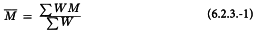
The products WM are formed for each assay and their sum divided by the total weight for all assays to give the logarithm of the weighted mean potency.
The standard error of the ln (mean potency) is taken to be the square root of the reciprocal of the total weight:
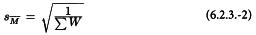
and approximate confidence limits are obtained from the antilogarithms of the value given by:

where the number of degrees of freedom of t equals the sum of the number of degrees of freedom for the error mean squares in the individual assays.
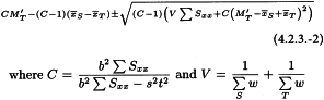
6.2.4. Weighted mean and confidence limits based on the intra- and inter-assay variation
When results of several repeated assays are combined, the (χ2-value may be significant. The observed variation is then considered to have two components:
 ,
,
where  is the unweighted mean. The former varies from assay to assay whereas the latter is common to all M.
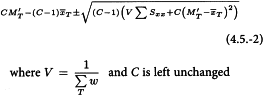
For each M a weighting coefficient is then calculated as:

which replaces W in Section 6.2.3. where t is taken to be approximately 2.
6.3. UNWEIGHTED COMBINATION OF ASSAY RESULTS
To combine the n′ estimates of M from n′ assays in the simplest way, the mean is calculated and an estimate of its standard deviation is obtained by calculating:
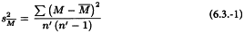
and the limits are:

where t has (n′- 1) degrees of freedom. The number n′ of estimates of M is usually small, and hence the value of t is quite large.
6.4. EXAMPLE OF A WEIGHTED MEAN POTENCY WITH CONFIDENCE LIMITS
Table 6.4.-I lists 6 independent potency estimates of the same preparation together with their 95 per cent confidence limits and the number of degrees of freedom of their error variances. Conditions 1, 2 and 3 in Section 6.2. are met. The ln potencies and the weights are calculated as described in Section 6.2.
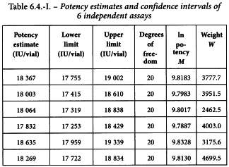
Homogeneity of potency estimates is assessed with formula 6.2.2.-1 which gives a χ2 of 4.42 with 5 degrees of freedom. This is not significant (p = 0.49) and thus all conditions are met.
A weighted mean potency is calculated with formula 6.2.3.-1 which yields 9.8085.
Formula 6.2.3.-2 gives a standard deviation of 0.00673 and approximate 95 per cent confidence limits of 9.7951 and 9.8218 are calculated with formula 6.2.3.-3 where t has 120 degrees of freedom.
By taking the antilogarithms a potency of 18 187 IU/vial is found with 95 per cent confidence limits from 17 946-18 431 IU/vial.
7. Beyond this annex
It is impossible to give a comprehensive treatise of statistical methods in a pharmacopoeial text. However, the methods described in this annex should suffice for most pharmacopoeial purposes. This section tries to give a more abstract survey of alternative or more general methods that have been developed. The interested reader is encouraged to further explore the existing literature in this area. The use of more specialised statistical methods should, in any case, be left to qualified personnel.
7.1. GENERAL LINEAR MODELS
The methods given in this annex can be described in terms of general linear models (or generalised linear models to include the probit and logit methods). The principle is to define a linear structure matrix X (or design matrix) in which each row represents an observation and each column a linear effect (preparation, block, column, dose). For example: the Latin square design in example 5.1.2 would involve a matrix with 36 rows and 13 columns. 1 column for each of the preparations, 1 column for the doses, 5 columns for each block except the first, and 5 columns for each row except the first. All columns, except the one for doses, are filled with 0 or 1 depending on whether or not the observation relates to the effect. A vector Y is filled with the (transformed) observations. The effects are estimated with the formula (XTX)-1XTY from which the potency estimate m can easily be derived as a ratio of relevant effects. Confidence intervals are calculated from Fieller′s theorem:
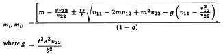
and v11, v22, v12 represent the variance multipliers for the numerator, the denominator and their covariance multiplier respectively. These are taken directly from (XTX)-1 or indirectly by noting that:

and 
A full analysis of variance in which all components are partitioned is slightly more complicated as it involves a renewed definition of X with more columns to relax the assumptions of parallelism and linearity, after which the linear hypotheses can be tested. For assays depending upon quantal responses the linear effects (intercepts aS, aT etc. and the common slope b are found by maximising the sum over treatments of nln Φ(ai + bx) + (n- R)ln(1 -Φ(ai + bx)) where x is the ln(dose), Φ denotes the shape of the distribution and i ∈ {S, T, ...}.
7.2. HETEROGENEITY OF VARIANCE
Heterogeneity of variance cannot always be solved by simply transforming the responses. A possible way to cope with this problem is to perform a weighted linear regression. In order to obtain an unbiased estimate, the weight of the observations is taken to be proportional to the reciprocal of the error variances. Since the true error variance is not always known, an iterative reweighted linear procedure may be followed. However, the calculation of the confidence interval involves new problems.
7.3. OUTLIERS AND ROBUST METHODS
The method of least squares described in this annex has the disadvantage of being very sensitive to outliers. A clear outlier may completely corrupt the calculations. This problem is often remedied by discarding the outlying result from the dataset. This policy can lead to arbitrary rejection of data and is not always without danger. It is not easy to give a general guideline on how to decide whether or not a specific observation is an outlier and it is for this reason that many robust methods have been developed. These methods are less sensitive to outliers because they give less weight to observations that are far away from the predicted value. New problems usually arise in computing confidence intervals or defining a satisfactory function to be minimised.
7.4. CORRELATED ERRORS
Absolute randomisation is not always feasible or very undesirable from a practical point of view. Thus, subsequent doses within a dilution series often exhibit correlated errors leading to confidence limits that are far too narrow. Some methods have been developed that take account of this autocorrelation effect.
7.5. EXTENDED NON-LINEAR DOSE-RESPONSE CURVES
Analysis of extended non-linear dose-response curves raises a number of statistical questions which require consideration, and for which professional advice is recommended. Some of these are indicated below.
1) An example using the four-parameter logistic function has been shown. However, models based on functions giving other sigmoid curves may also be used. Models incorporating additional asymmetry parameters have been suggested.
2) Heterogeneity of variance is common when responses cover a wide range. If the analysis ignores the heterogeneity, interpretation of results may not be correct and estimates may be biased. Use of the reciprocal of the error variances as weights is unlikely to be reliable with limited numbers of replicates. It may be appropriate to estimate a function which relates variance to mean response.
3) The statistical curve-fitting procedures may give different estimates depending on assumptions made about the homogeneity of the variance and on the range of responses used.
4) In principle, equality of upper and lower response limits for the different preparations included in an assay can be directly tested in each assay. However, interpretation of the results of these tests may not be straightforward. The tests for linearity and parallelism given by the simplified method of analysis (Example 5.4.1) indirectly incorporate tests for equality and accuracy of upper and lower limits.
5) Many assays include “controls” which are intended to identify the upper and/or lower response limits. However, these values may not be consistent with the statistically fitted upper and lower response limits based on the extended dose-response curve.
6) The simplified method of analysis given in Example 5.4.1 provides approximate confidence intervals. Other methods may also be used, for example intervals based on lack-of-fit of the completely specified model. For typical assay data, with responses covering the complete range for each preparation tested, all methods give similar results.
7.6. non-parallelism of dose-response curves
Similarity of dose-response relationships is a fundamental criterion for assessing whether an assay may be regarded as a dilution assay and hence whether the estimation of relative potency is valid (see Section 3.1.1).
This criterion is frequently met by showing that dose-response curves for standard and test samples do not deviate significantly from parallelism. Underestimation of the residual error can lead to excess rejection of assays due to significant deviations from parallelism and/or linearity. This is often an artefact of inappropriate assay design or analysis. Minor modifications to assay designs might in many cases substantially improve the estimation of the residual error. Analysis allowing for the actual level of replication may also improve the situation, e.g. by accounting for multiple applications of the same dilution or correlation of errors between serial dilutions. If estimation of the relevant residual error is not feasible for individual assays, for example because it is impractical to create independent doses and/or replicates, it might be possible to obtain a more correct estimate of the residual error during the assay validation process. In such a case it may be justified to replace the residual error, estimated from the individual assay, by an average (pooled) residual error, determined during the validation process and agreed by the competent authorities.
Where not specified by relevant procedures, curve similarity may be assessed by another approach described as “equivalence testing”, whereby, during the validation process, a range of the allowable difference between slopes or other measures of curve similarity, an equivalence acceptance criterion, is determined. If supported by appropriate documentation and agreed by the competent authorities, meeting the equivalence acceptance criteria may be used to satisfy the curve similarity requirement.
There may be cases where the assay system is sufficiently precise to detect genuine non-parallelism. If there is true non-parallelism this needs to be recognised and a suitable solution adopted. A solution might, for example, require a suitable standard that is similar in composition to, and therefore parallel to, the test samples. If the assay system is responding in a non-specific manner to extraneous components of the standard or test samples, then a more specific assay system that does not respond to the irrelevant components may be the solution. No simple, generally applicable statistical solution exists to overcome these fundamental problems. The appropriate action has to be decided on a case-by-case basis with the help of statistical expertise.
8. Tables and generating procedures
The tables in this section list the critical values for the most frequently occurring numbers of degrees of freedom. If a critical value is not listed, reference should be made to more extensive tables. Many computer programs include statistical functions and their use is recommended instead of the tables in this section. Alternatively, the generating procedures given below each table can be used to compute the probability corresponding to a given statistic and number of degrees of freedom.
8.1. The F-distribution
If an observed value is higher than the value in Table 8.1.-I, it is considered to be significant (upper lines, p = 0.05) or highly significant (lower lines, p = 0.01). df1 is the number of degrees of freedom of the numerator and df2 is the number of degrees of freedom of the denominator.
Generating procedure Let F be the F-ratio and df1 and df2 as described above. Let pi = π = 3.14159265358979... The procedure in Table 8.1.-II will then generate the p-value.
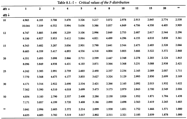

8.2. The t-distribution
If an observed value is higher than the value in Table 8.2.-I, it is considered to be significant (p = 0.05) or highly significant (p = 0.01).
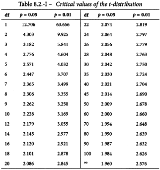
Generating procedures The p-value for a given t with df degrees of freedom can be found with the procedures in Section 8.1 where F = t2, df1 = 1 and df2 = df.
The t-value (p = 0.05) for a given number of degrees of freedom df can be found with the procedure in Table 8.2.-II, which should be accurate up to 6 decimal places.
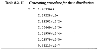
8.3. The χ2-distribution
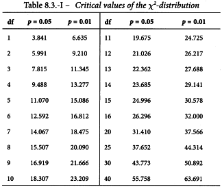
If an observed value is higher than the value in Table 8.3.-I, it is considered to be significant (p = 0.05) or highly significant (p = 0.01).
Generating procedure Let X2 be the χ2-value and df as described above. The procedure in Table 8.3.-II will then generate the p-value.
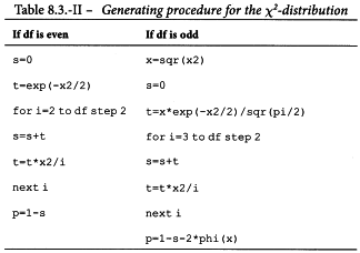
In this procedure phi is the cumulative standard normal distribution function Φ (see Section 8.4).
8.4. The Φ-distribution (The cumulative standard normal distribution)
The Φ-value for negative x is found from Table 8.4.-I as 1 - Φ(-x).
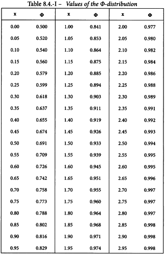
Generating procedure Let x be the x-value. The procedure in Table 8.4.-II will generate the corresponding Φ-value if 0 ≤ x ≤ 8.15. If x is greater than 8.15 the Φ-value can be set to 1. If x is negative, the formula given above can be used. This procedure assumes that the computer can represent about 15 decimal places. If less digits or more digits can be represented, the procedure needs some trivial modifications.

8.5. Random permutations
Random permutations are needed in randomised block designs. The following algorithm shows how the built-in random generator of a computer can be used to create random permutations of N treatments.
Step 1. Write the N possible treatments down in a row.
Step 2. Obtain a random integer R such that 1≤ R ≤ N.
Step 3. Exchange the r-th treatment with the N-th treatment in the row.
Step 4. Let N = N- 1 and repeat steps 2 to 4 until N = 1.
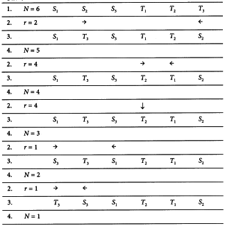
An example with 6 treatments will illustrate this algorithm.
8.6. Latin squares
The following example shows how 3 independent permutations can be used to obtain a Latin square.
1) Generate a random permutation of the N possible treatments (see Section 8.5):

2) A simple Latin square can now be constructed by “rotating” this permutation to the right. This can be done as follows. Write the permutation found in step 1 down on the first row. The second row consists of the same permutation, but with all treatments shifted to the right. The rightmost treatment is put on the empty place at the left. This is repeated for all the rows until all the treatments appear once in each column:
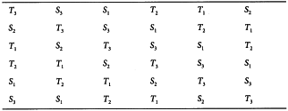
3) Generate 2 independent random permutations of the figures 1 to N:


4) The Latin square can now be found by sorting the rows and columns of the simple Latin square according to the 2 permutations for the rows and columns:
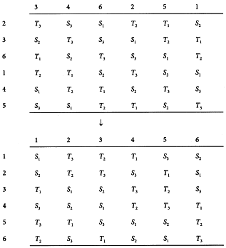
9. Glossary of symbols
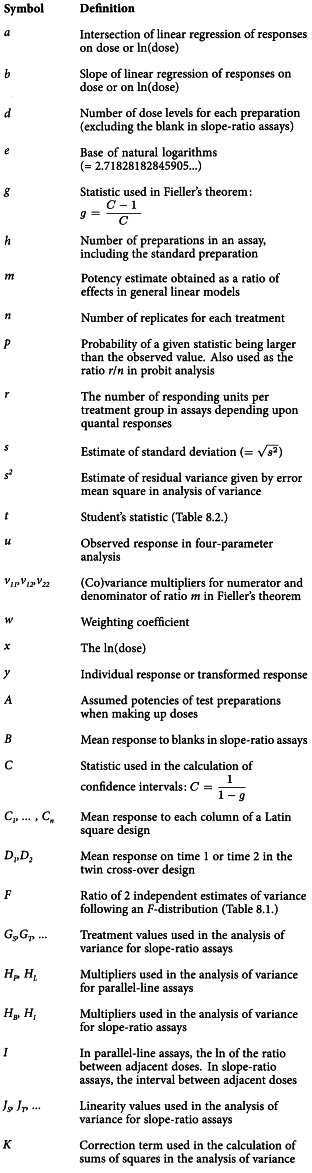
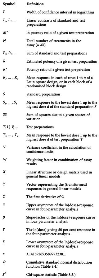
10. Literature
This section lists some recommended literature for further study.
Finney, D.J. (1971). Probit Analysis, 3rd Ed. Cambridge University Press, Cambridge.
Nelder, J.A. Wedderburn, R.W.M. (1972). Generalized linear models, Journal of the Royal Statistical Society, Series A 135, 370-384.
DeLean, A., Munson, P.J., and Rodbard, D. (1978). Simultaneous analysis of families of sigmoidal curves: Application to bioassay, radioligand assay, and physiological dose-response curves, Am. J. Physiol. 235(2): E97-E102.
Finney, D.J. (1978). Statistical Method in Biological Assay, 3rd Ed. Griffin, London.
Sokal, R.R. Rohlf, F.R. (1981). Biometry: Principles and Practice of Statistics in Biological Research, 2nd Ed. W.H. Freemann CO, New York.
Peace, K.E. (1988). Biopharmaceutical Statistics for Drug Development, Marcel Dekker Inc., New York/Basel.
Bowerman, B.L. O′Connell, R.T. (1990). Linear Statistical Models an Applied Approach, 2nd Ed. PWS-KENT Publishing Company, Boston.
Govindarajulu, Z. (2001). Statistical Techniques in Bioassay, 2nd revised and enlarged edition, Karger, New York.