SC IV R. Chemometric Methods Applied to Analytical Data

(Ph. Eur. general text 5.21)

The following chapter is published for information only. It is an introduction to the use of chemometric techniques for processing analytical data sets. The objective is to provide indications on good chemometric practice and requirements.

1 GENERAL ASPECTS

1-1 INTRODUCTION

1-1-1 Scope of the chapter

This chapter is an introduction to the use of chemometric techniques for the processing of analytical data sets, which is an area of interest for research, quality control and manufacturing in the pharmaceutical industry. The objective is to provide information on the requirements for good chemometric practice and to also present a selection of established chemometric methods, but not an exhaustive review of these techniques, as refinements and innovations are constantly being introduced. The principles of the proposed methods will be briefly described along with their critical aspects and limitations. Mathematical details and algorithms are mostly omitted and a glossary is provided at the end of the chapter.

1-1-2 Definition

The actual definition of chemometrics is “the chemical discipline that uses mathematical and statistical methods, (a) to design or select optimal measurement procedures and experiments, and (b) to provide maximum chemical information by analysing chemical data”.

From a more general point of view, chemometrics is not limited to chemical data and can contribute greatly to system understanding by analysing data, when limited knowledge and theory do not sufficiently explain observations and behaviour. Chemometric methods consist mainly of multivariate data-driven modelling techniques that result in empirical mathematical models that are subsequently used for the indirect prediction of properties of interest.

1-1-3 Background

Applications of chemometrics can be qualitative or quantitative, and it can help the analyst to structure the data set and to recognise hidden variable relationships within the system. However, it should be stressed that although such data-driven methods may be powerful, they would not replace a verified or established theory if available.

Chemometric methods have revolutionised near infrared spectroscopy (NIR) and such techniques are now integral components of process analytical technology (PAT) and quality by design (QbD) for use in improved process monitoring and quality control in a variety of fields. Chemometric methods can be found throughout the scientific and technological community, with a principal but non-exclusive focus on life and health sciences such as agriculture, food, pharmacy, chemistry, biochemistry and genomics, but also other industries such as oil, textiles, sensorics and cosmetics, with the potential to expand even further into other domains.

The associated mathematical principles have been understood since the early twentieth century, but chemometrics came of age with the development of digital technology and the related progress in the elaboration of mathematical algorithms. Many techniques and methods are based on geometric data representations, transformations and modelling. Later, mathematical and theoretical developments were also consolidated.

1-1-4 Introducing chemometrics

In chemometrics, a property of interest is evaluated solely in terms of the information contained in the measured samples. Algorithms are applied directly to the data set, and information of interest is extracted with models (modelling or calibration step). Chemometrics is associated with multivariate data analysis, which usually depends less on assumptions about the distribution of the data than many other statistical methods since it rarely involves hypothesis testing. During modelling the most sensitive changes in properties of interest can be amplified, while the less relevant changes in disturbing factors, whatever their origin, i.e. physical, chemical, experimental or instrumental variation, are minimised to the level of noise.

A model in chemometrics is a prediction method and not a formal or simplified representation of a phenomenon from physics, chemistry, etc. The ability of a model to predict properties has to be assessed with regard to its performance. The best model or calibration will provide the best estimations of properties of interest. A useful model is one that can be trusted and used for decision-making, for example. Adoption of a model in decision-making must be based on acceptable, reliable, and well-understood assessment procedures.

In univariate analysis, identified variables in a system are analysed individually. However, in reality, systems tend to be more complex, where interactions and combination effects occur between sample variables and cannot be separated. Multivariate data analysis handles many variables simultaneously and the relationship within or between data sets (typically matrices) has to be rearranged to reveal the relevant information. In multivariate methods, the original data is often combined linearly to account as much as possible for the explainable part of the data and ideally, only noise will remain unmodelled. The model, when properly validated, can be used in place of costly and time-consuming measurements in order to predict new values.

Generally, projection techniques such as principal components analysis (PCA), principal components regression (PCR) or partial least squares regression (PLS) are recommended. However, the approach will be different depending on whether the data has been generated using experimental design (i.e. designed data) or has been collected at random from a given population (i.e. non-designed data). With designed data matrices, the variables are orthogonal by construction and traditional multilinear statistical methods are therefore well suited to describing the data within. However, in non-designed data matrices, the variables are seldom orthogonal, but are more or less collinear, which favours the use of multivariate data analysis.

1-1-5 Qualitative and quantitative data analysis

Qualitative data analysis can be divided into exploration, an unsupervised analysis where data from a new system is to be analysed, and classification, a supervised analysis where class-labels are predicted.

Unsupervised analysis

In exploratory data analysis, multivariate tools are used to gather an overview of the data in order to build hypotheses, select suitable analytical methods and sampling schemes, and to determine how multivariate analysis of current and future data of similar type can be performed. When the first exploratory treatment is finalised, classification can be subsequently carried out in the form of a secondary treatment, where samples are organised into specific groups or classes.

Supervised analysis

Classification is the process of determining whether or not samples belong to the same class as those used to build the model. If an unknown sample fits a particular model well, it is said to be a member of that class. Many analytical tasks fall into this category, e.g. materials may be sorted according to quality, physical grade and so on. Identity testing is a special situation where unknown samples are compared with suitable reference materials, either by direct comparison or indirect estimation, e.g. using a chemometric model.

Quantitative data analysis, on the other hand, mainly consists of calibration, followed by direct application to new and unknown samples. Calibration consists of predicting the mathematical relationship between the property to be evaluated (e.g. concentration) and the variables measured.

1-2 GOOD CHEMOMETRIC PRACTICE

The following notation will be used in the chapter:

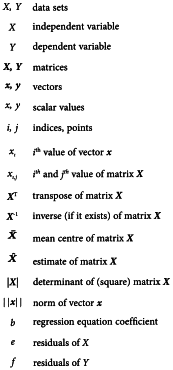
1-2-1 Figures of merits for regression

In quantitative analysis, building a regression model involves fitting a mathematical relationship to the corresponding independent data (X) and dependent data (Y). The independent data may represent a collection of signals, i.e. responses from a number of calibration samples, while the dependent data may correspond to the values of an attribute, i.e. the property of interest in the calibration samples. It is advisable to test the regression model with internal and external test sets. The internal test set consists of samples that are used to build the model (or achieve calibration) by applying resampling within the calibration data and samples that are initially left out of the calibration in order to validate the model. Use of the internal test set is part of model optimisation and model selection. The external independent test set represents data that normally is available after the model has been fixed, thus the external test set challenges the model and tests its robustness for the analysis of future data.

1-2-1-1 Root mean square error of prediction

The link between X and Y is explored through a common set of samples (calibration set) from which both x and y-values have been collected and are clearly known. For a second set of samples (validation set) the predicted y-values are then compared to the reference y-values, resulting in a prediction residual that can be used to compute a validation residual variance, i.e. a measure of the uncertainty of future predictions, which is referred to as root mean square error of prediction (RMSEP). This value estimates the uncertainty that can be expected when predicting y-values for new samples. Since no assumptions concerning statistical error distribution are made during modelling, prediction error cannot be used to report a valuable statistical interval for the predicted values. Nevertheless, RMSEP is a good error estimate in cases where both calibration and validation sample sets are representative of future samples.

A confidence interval for predicted y-values would be ± n × RMSEP, with n fixed by the operator. A common choice is n = 2. This choice should be dependent on the requirements of the specific analytical method.

Chemometric models can end up with better precision than the reference methods used to acquire calibration and testing data. This is typically observed for water content determinations by NIR and PLS where semi-micro determination titration (2.5.12) is the reference method.

1-2-1-2 Standard error of calibration and coefficient of determination

Figures of merit can be calculated to help assess how well the calibration fits the data. Two examples of such statistical expressions are the standard error of calibration (SEC) and the coefficient of determination (R²).

SEC has the same units as the dependent variables and reflects the degree of modelling error, but cannot be used to estimate future prediction errors. It is an indication of whether the calculation using the calibration equation will be sufficiently accurate for its intended purpose. In practice SEC has to be compared with the error of the reference method (SEL, Standard Error of Laboratory, see Glossary). Usually SEC is larger than SEL, in particular if modelling does not account for all interferences in the samples or if other physical phenomena are present.

The coefficient of determination (R²) is a dimensionless measure of how well the calibration fits the data. R² can have values between 0 and 1. A value close to 0 indicates that the calibration fails to relate the data to the reference values and as the coefficient of determination increases, the X-data becomes an increasingly more accurate predictor of the reference values. Where there is more than 1 independent variable, adjusted R² should be used rather than R², since the number of independent variables in the model inflates the latter even if the fraction of variance explained by the model is not increased.

1-2-2 Implementation steps

The implementation of chemometric methods varies case by case depending on the specific requirements of the system to be analysed. The following generic approach can be followed when analysing non-designed data sets:

— in formulating the study problem, define the precise objective of data collection and the expected analysis results;

— investigate the origin and availability of the data. The data set should cover the variation of the explored variable(s) or attribute(s);

— if the available data does not cover the expected variation, prepare and measure samples that fill the gap;

— variable selection: sometimes selecting the right variables can give more robustness and also enhance model accuracy;

— raw data may have to be transformed and mathematical pre-treatments performed;

— elaborate the model through calibration and validation;

— challenge the model and check its performance on new samples or data;

— validate the method according to current pharmaceutical usage and requirements.

1-2-3 Data considerations

1-2-3-1 Sample quality

Careful sample selection increases the likelihood of extracting useful information from the analytical data. Whenever it is possible to actively adjust selected variables or parameters according to an experimental design, the quality of the results is increased. Experimental design (also referred to as design of experiments, DoE) can be used to introduce systematic and controlled changes between samples, not only for analytes, but also for interferences. When modelling, common considerations include the determination of which variables are necessary to adequately describe the samples, which samples are similar to each other and whether the data set contains related sub-groups.

1-2-3-2 Data tables, geometrical representations

Sample responses result in a group of numerical values relating to signal intensities (X-data), i.e. the independent variables. However, it should be recognised that these variables are not necessarily linearly independent (i.e. orthogonal) according to mathematical definitions. These values are best represented in data tables and by convention each sample is associated with a specific row of data. A collection of such rows constitutes a matrix, where the columns are the variables. Samples can then be associated with certain features reflecting their characteristics, i.e. the value of a physical or chemical property or attribute and these data are usually referred to as the Y-data, i.e. the dependent variables. It is possible to add this column of values to the sample response matrix, thereby combining both the response and the attribute of each sample.

When n objects are described by m variables the data table corresponds to an n×m matrix. Each of the m variables represents a vector containing n data values corresponding to the objects. Each object therefore appears as a point in an m dimensional space described by its m coordinate values (1 value for each variable in the m axes).

1-2-3-3 First assessment of data

Before performing multivariate data analysis, the quality of the sample response can be optionally assessed using statistical tools. Graphical tools are recommended for the 1^st visual assessment of the data, e.g. histograms and/or boxplots for variables for evaluation of the data distribution, and scatter plots for detection of correlations. Descriptive statistics are useful for obtaining a rapid evaluation of each variable, taken separately, before starting multivariate analysis. For example, mean, standard deviation, variance, median, minimum, maximum and lower/upper quartile can be used to assess the data and detect out-of-range values and outliers, abnormal spread or asymmetry. These statistics reveal anomalies in a data table and indicate whether a transformation might be useful or not. Two-way statistics, e.g. correlation, show how variations in 2 variables may correlate in a data table. Verification of these statistics is also useful when reducing the size of the data table, as they help in avoiding redundancies.

1-2-3-4 Outliers

An outlier is a sample that is not well described by the model. Outliers can be X or Y in origin. They reflect unexpected interference in the original data or measurement error. The predicted data that is very different from the expected value calls into question the suitability of the modelling procedure and the range spanned by the original data. In prediction mode, outliers can be caused by changes in the interaction between the instrument and samples or if samples are outside the model’s scope. If this new source of variability is confirmed and is relevant, the corresponding data constitutes a valuable source of information. Investigation is recommended to decide whether the existing calibration requires strengthening (updating) or whether the outliers should be ignored as uncritical or unrelated to the process (i.e. operator error).

In the case of classification an outlier test should be performed on each class separately.

1-2-3-5 Data error

Types of data error include random error in the reference values of the attributes, random error in the collected response data and systematic error in the relationship between the two. Sources of calibration error are problem specific, for example, reference method errors and errors due to either sample non-homogeneity or the presence of non-representative samples in the calibration set. Model selection during calibration usually accounts for only a fraction of the variance or error attributable to the modelled analytical technique. However, it is difficult to assess if this error is more significant than the reference method error or vice versa.

1-2-3-6 Pre-processing and variable selection

The raw data may not be optimal for analysis and are generally pre-processed before performing chemometric calculations to improve the extraction of physical and chemical information.

Interferences, for example background effects, baseline shifts and measurements in different conditions, can impede the extraction of information when using multivariate methods. It is therefore important to minimise the noise introduced by such effects by carrying out pre-processing operations.

A wide range of transformations (scaling, smoothing, normalisation, derivatives, etc.) can be applied to X-data as well as Y-data for pre-processing prior to multivariate data analysis in order to enhance the modelling. The main purpose of these transformations is focussing the data analysis on the pertinent variability within the data set. For example, pre-processing may involve mean centering of variables so that the mean does not influence the model and thus reduce the model rank.

The selection of the pre-processing is mostly driven by parameters such as type of data, instrument or sample, the purpose of the model and user experience. Pre-processing methods can be combined, for example standard normal variate (SNV) with 1st derivative, as an empirical choice.

1-2-4 Maintenance of chemometric models

Chemometric methods should be reassessed regularly to demonstrate a consistent level of acceptable performance. In addition to this periodical task, an assessment should be carried out for critical parameters when changes are made to application conditions of the chemometric model (process, sample sources, measurement conditions, analytical equipment, software, etc.).

The aim of maintaining chemometric models up-to-date is to provide applications that are reliable over a longer period of use. The extent of the validation required, including the choice of the necessary parameters, should be based on risk analysis, taking into account the analytical method used and the chemometric model.

1-3 ASSESSMENT AND VALIDATION OF CHEMOMETRIC METHODS

1-3-1 Introduction

Current use of the term ‘validation’ refers to the regulatory context as applied to analytical methods, but the term is also used to characterise a typical computation step in chemometrics. Assessment of a chemometric model consists of evaluating the performance of the selected model in order to design the best model possible with a given set of data and prerequisites. Provided sufficient data are available, a distribution into 3 subsets should always be considered: 1) a learning set to elaborate models, 2) a validation set to select the best model, i.e. the model that enables the best predictions to be made, 3) an independent test set to estimate objectively the performance of the selected final model. Introducing a 3^rd set for objective model performance evaluation is necessary to estimate the model error, among other performance indicators. An outline is given below on how to perform a typical assessment of a chemometric model, starting with the initial validation, followed by an independent test validation and finally association/correlation with regulatory requirements.

1-3-2 Assessment of chemometric models

1-3-2-1 Validation during modelling

Typically, algorithms are iterative and perform self-optimisation during modelling through an on-going evaluation of performance criteria and figures of merit. This step is called validation. The performance criteria are specific to the chemometric technique used and to the nature of the analytical data, as well as the purpose of the overall method which includes both the analytical side and the chemometric model. The objective of the validation is to evaluate the model and provide help to select the best performing model. Selected samples are either specifically assigned for this purpose or are selected dynamically through reselection/re-use of data from a previous data set (sometimes called resampling – for clarification, see Glossary). A typical example of data reselection is cross-validation with specific segments, for example ‘leave-one-out’ cross-validation when samples are only a few, or ‘leave-subset-out’ cross-validation (Figure 5.21.-1). Another type of resampling is bootstrapping.

Figure 5.21.-1. – Cross-validation with leave subset of 3 out applied to linear regression. Regression model data = ●. Subset used for test =○. The errors of fit (interrupted lines) are collected to form the cumulated cross-validation error

1-3-2-2 Assessment of the model

Once the model matches the optimisation requirements, fitness for purpose is assessed. Independent samples not used for modelling or model optimisation are introduced at this stage as an independent test-set in order to evaluate the performance of the model. Ideally, when sufficient data are available, the sample set can be split into 3 subsets comprising 1 learning set for model computation, 1 validation set for optimisation of the model, and 1 test set for evaluation of the prediction ability, i.e. whether the model is fit for purpose. The 3 subsets are treated independently and their separation should be performed in such a way that model computation is not biased. The aim is to obtain a representative distribution of the samples within the 3 subsets with regard to their properties and expected values.

1-3-2-3 Size and partitioning of data sets

The size of the data set needed for building the calibration is dependent on the number of analytes and interfering properties that needs to be handled in the model. The size of the learning data set for calibration usually needs to be larger when the interfering variations are acquired randomly than when all major interferences are known and they can be varied according to a statistical experimental design. The lowest possible number of samples needed to cover the calibration range can be estimated from the corresponding design. The size of the independent test set should be in the order of 20-40 per cent of the samples used for the calibration model. However, when representative samples are abundant, the larger the test data set (above 40 per cent), the more reliably the prediction performance can be estimated. It is common practice to mix learning and model validation sets and as a result, the definitive assessment of the model relies on the separate test set.

1-3-3 Validation according to the regulatory framework

Validation principles and considerations are described in established international guidelines and apply to the validation of analytical methods. However, due to the special nature of data treatment and evaluation, as carried out in most chemometric methods, additional aspects have to be taken into account when validating analytical procedures. In this context, validation comprises both the assessment of the analytical method performance and the evaluation of the model. In some special cases, it might only be necessary to validate the chemometric model (see section 1-2-4).

1-3-3-1 Qualitative models

For validation of qualitative models, the most critical parameters are specificity and robustness. When not applicable, scientific justification is required.

Specificity

During validation it has to be shown that the model possesses sufficient discriminatory capability. Therefore, a suitable set of materials that pose a risk of mix-up must be defined and justified. If, in addition to chemical identification, other parameters (such as polymorphism, particle size, moisture content, etc.) are relevant, a justification for these parameters should also be included. The selection of materials to be included when validating specificity should be based on logistic considerations (e.g. materials handled close to the process under review, especially those with similar appearance), chemical considerations (e.g. materials with similar structure) and also physical considerations where relevant (e.g. materials with different physical properties). After definition of this set of materials, the discriminatory ability of the chemometric method to reject them must be proven. Therefore, for each material a representative set of samples covering typical variance within the material has to be analysed and evaluated. If the specificity of the chemometric model is insufficient, the parameters of the model should be optimised accordingly and the method revalidated.

Whenever new elements that may potentially affect identification are introduced, e.g. new materials that are handled at the same site and represent a risk of mix-up, a revalidation of specificity should be carried out. This revalidation can be limited to the new element and does not necessarily need to encompass the complete set of elements, whose constituents may not all be affected by the change.

If properties of materials change over time (e.g. batches of materials with lower or higher particle size, lower or higher moisture content etc.) and these changes become relevant, they should also be included as part of the validation. This can be achieved for example, by an amendment to the validation protocol and does not necessarily require a complete revalidation of the chemometric model.

To assess specificity, the number of false-positive and false-negative errors can be evaluated by classification of the test set.

Robustness

For validation of robustness, a comprehensive set of critical parameters (e.g. process parameters such as temperature, humidity, instrumental performance of the analytical equipment) should be considered. The reliability of the analytical method should be challenged by variation of these parameters. It can be advantageous to use experimental design (DoE) to evaluate the method.

To assess robustness the number of correct classifications, correct rejections, false-positive and false-negative errors can be evaluated by classification of samples under robustness conditions.

1-3-3-2 Quantitative models

The following parameters should be addressed unless otherwise justified: specificity, linearity, range, accuracy, precision and robustness.

Specificity

It is important to detect that the sample that is quantified is not an outlier with respect to the calibration space. This can be done using the correlation coefficient between the sample and the calibration mean, as well as Hotelling T² among others.

Linearity

Linearity should be validated by correlating results from the chemometric model with those from an analytical reference method. It should cover the entire range of the method and should involve a specifically selected set of samples that is not part of the calibration set. For orientation purposes, a ‘leave-subset-out’ cross-validation based on the calibration set may be sufficient, but should not replace assessment using an independent test set. Linearity can be evaluated through the correlation coefficient, slope and intercept.

Range

The range of analyte reference values defines the range of the chemometric model, and its lower limit determines the limits of detection and quantification of the analytical method. Controls must be in place to ensure that results outside this range are recognised as such and identified. Within the range of the model, acceptance criteria for accuracy and precision have to be fulfilled.

Accuracy

The accuracy of the chemometric model can be determined by comparison of analytical results obtained from the chemometric model with those obtained using a reference method. The evaluation of accuracy should be carried out over the defined range of the chemometric model using an independent test set. It may also be helpful to assess the accuracy of the model using a ‘leave-subset-out’ cross-validation, although, this should not replace assessment using an independent test set.

Precision

The precision of the analytical method should be validated by assessing the standard deviation of the measurements performed through the chemometric model. Precision covers repeatability (replicate measurements of the same sample by the same person on the same day) and intermediate precision (replicate measurements of the same sample by another person on different days). Precision should be assessed at different analyte values covering the range of the chemometric model, or at least at a target value.

Robustness

For validation of robustness, the same principles as described for qualitative methods apply. Extra care should be taken to investigate the effects of any parameters relevant for robustness on the accuracy and precision of the chemometric model. It can be an advantage to evaluate these parameters using experimental design.

The chemometric model can also be investigated using challenge samples, which may be samples with analyte concentrations outside the range of the method or samples of different identity. During the validation, it must be shown that these samples are clearly recognised as outliers.

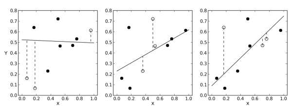
2 CHEMOMETRIC TECHNIQUES

A non-exhaustive selection of chemometric methods are discussed below. A map of the selected methods is given in Figure 5.21.-2.

Figure 5.21.-2. – Map of chemometric methods discussed in the chapter

2-1 PRINCIPAL COMPONENTS ANALYSIS

2-1-1 Introduction

The complexity of large data sets or tables makes human interpretation difficult without supplementary methods to aid in the process. Principal components analysis (PCA) is a projection method used to visualise the main variation in the data. PCA can show in what respect 1 sample differs from another, which variables contribute most to this difference and whether these variables contribute in the same way and are correlated or are independent of each other. It also reveals sample set patterns or groupings within the data set. In addition, PCA can be used to estimate the amount of useful information contained in the data table, as opposed to noise or meaningless variations.

2-1-2 Principle

PCA is a linear data projection method that compresses data by decomposing it to so-called latent variables. The procedure yields columns of orthogonal vectors (scores), and rows of orthonormal vectors (loadings). The principal components (PCs), or latent variables, are a linear combination of the original variable axes. Individual latent variables can be interpreted via their connection to the original variables. In essence, the same data is shown but in a new coordinate system. The relationships between samples are revealed by their projections (scores) on the PCs. Similar samples group together in respect to PCs. The distance between samples is a measure of similarity/dissimilarity.

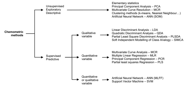
The original data table is transformed into a new, rearranged matrix whose structure reveals the relationships between rows and columns that may be hidden in the original matrix (Figure 5.21.-3). The new structure constitutes the explained part of the original data. The procedure models the original data down to a residual error, which is considered the unexplained part of the data and is minimised during the decomposition step.

The underlying idea is to replace a complex data table with a simpler counterpart version having fewer dimensions, but still fitting the original data closely enough to be considered a good approximation (Figure 5.21.-4). Extraction of information from a data table consists of exploring variations between samples, i.e. finding out what makes a sample different from or similar to another. Two samples can be described as similar if they have similar values for most variables. From a geometric perspective, the combination of measurements for 1 sample defines a point in a multidimensional space with as many dimensions as there are variables. In the case of close coordinates the 2 points are located in the same area or volume. With PCA, the number of dimensions can be reduced while keeping similar samples close to each other and dissimilar samples further apart in the same way as in the multidimensional space, but compressed into an alternate lower dimensional coordinate system.

The principle of PCA is to find the directions in the data space that describe the largest variation of the data set, i.e. where the data points are furthest apart. Each direction is a linear combination of the initial variables that contribute most to the actual variation between samples. By construction, principal components (PCs) are orthogonal to each other and are also ranked so that each carries more information than any of those that follow. Priority is therefore given to the interpretation of these PCs, starting with the 1^st, which incorporates the greatest variation and thereby constitutes an alternative less complex system that is more suitable for interpreting the data structure. Normally, only the 1^st PCs contain pertinent information, with later PCs being more likely to describe noise. In practice, a specific criterion is used to ensure that noise is not mistaken for information and this criterion should be used in conjunction with a method such as cross-validation or evaluation of loadings in order to determine the number of PCs to be used for the analysis. The relationships between samples can then be subsequently viewed in 1 or a series of score plots. Residuals Ê keep the variation that is not included in the model, as a measure of how well samples or variables fit that model. If all PCs were retained, there would be no approximation at all and the gain in simplicity would consist only of ordering the variation of the PCs themselves by size. Deciding on the number of components to retain in a PCA model is a compromise between simplicity, robustness and goodness of fit/performance.

2-1-3 Assessment of model

Total explained variance R² is a measure of how much of the original variation in the data is described by the model. It expresses the proportion of structure found in the data by the model. Total residual and explained variances show how well the model fits the data. Models with small total residual variance (close to 0 per cent) or large total explained variance (close to 100 per cent) can explain most of the variation in the data. With simple models consisting of only a few components, residual variance falls to 0; otherwise, it usually means that the data contains a large amount of noise. Alternatively, it can also mean that the data structure is too complex to be explained using only a few components. Variables with small residual variance and large explained variance for a particular component are well defined by the model. Variables with large residual variance for all or the 1^st components have a small or moderate relationship with other variables. If some variables have much larger residual variance than others for all or the 1^st components, they may be excluded in a new calculation and this may produce a model that is more suitable for its purpose. Independent test set variance is determined by testing the model using data that was not used in the actual building of the model itself.

Figure 5.21.-3. – Geometrical representation of 3 different X-data sets. On the left, objects are plotted in the multivariate space, and the following examples reveal a hidden structure, i.e. a plane and a line respectively

Figure 5.21.-4. – Decomposition of the X-matrix for principal components analysis (PCA)

2-1-4 Critical aspects

PCA catches the main variation within a data set. Thus comparatively smaller variations may not be distinguished.

2-1-5 Potential use

PCA is an unsupervised method, making it a useful tool for exploratory data analysis. It can be used for visualisation, data compression, checking groups and trends in the data, detecting outliers, etc.

For exploratory data analysis, PCA modelling can be applied to the entire data table once. However, for a more detailed overview of where a new variation occurs, evolving factor analysis (EFA) can be used and, in this case, PCA is applied in an expanding or fixed window, where it is possible to identify, for example, the manifestation of a new component from a series of consecutive samples.

PCA also forms the basis for classification techniques such as SIMCA and regression methods such as PCR. The property of PCA to capture the largest variations in the 1^st principal components allows subsequent regression to be based on fewer latent variables. Examples of utilising components as independent data in regression are PCR, MCR, and ANN.

PCA is used in multivariate statistical process control (MSPC) to combine all available data into a single trace and to apply a signature for each unit operation or even an entire manufacturing process based on, for example, Hotelling T² statistics, PCA model residuals or individual scores. In addition to univariate control charts, 1 significant advantage with PCA is that it can be used to detect multivariate outliers, i.e. process conditions or process output that has a different correlation structure than the one present in the previously modelled data.

2-2 MEASURES BETWEEN OBJECTS

The primary use of the following algorithms is to measure the degree of similarity between an object and a group or the centre of the data.

2-2-1 Similarity measures

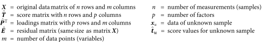
Calculation of the correlation is the simplest statistical tool used to compare data and to determine the degree of similarity, provided the data sets have the same dimension, e.g. spectral data. It is a measure of the linear association between a pair of vectors. A correlation score between -1 and +1 is calculated for the match, based on the system below, where a perfect match (mirror image) would have a score of +1 and 2 lines that are complete opposites would have a score of -1 (Figure 5.21.-5).

Figure 5.21.-5. – Examples of correlation scores illustrated by matching of the shapes

Correlation is used to compare data sets in any of the following ways:

— comparison of 2 selected samples;

— comparison of 1 or more selected samples represented by vectors with a reference data library (from a group or class).

The reference data can be the average of a group of typical characteristics.

Correlation r between 2 vectors x and y of the same dimension can be calculated using the following equation:

2-2-2 Distance measures

In the object space, a collection of objects will be seen as points that are more or less close to each other and will gather into groups or clusters. Measuring the distance between points will express the degree of similarity between objects. In the same way, measuring the distance of a point to the centre of a group will give information about the group membership of this object. The following algorithms are given to illustrate the way objects can be compared.

2-2-2-1 Euclidean distance

The Euclidean distance ed_i,j between 2 points i and j can be calculated as:

Similarly, the Euclidean distance ed_i,c between the point i and the centre c of the data can be calculated as the square root of the sum of the squared differences of the coordinates of point i to the mean value of the x-coordinates for each of the m axes, which can be expressed by the following matrix notation:

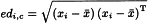
where x_i denotes the m values of coordinates describing the point i and x̄ denotes the mean coordinates calculated for the m variables. The superscript T indicates that the 2^nd term of the equation is transposed.

2-2-2-2 Mahalanobis distance

The Mahalanobis distance (md) takes into account the correlation between variables by using the inverse of the variance-covariance matrix:

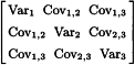
The variance-covariance matrix C_x is calculated using the following equation:

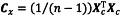
where X_c is the n×m data matrix centred over the mean of each column. Thus C_x is a square matrix that contains the variance of each variable over its diagonal and the covariance between variables on both sides of the diagonal. The Mahalanobis distance of point i to the centre c of the data is given by the following equation:

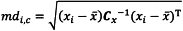
The C_x^-1 matrix is the inverse of the variance-covariance matrix and C_xC_x^-1 = I, where I is the identity matrix. The number of variables or principal components involved in calculating the distance is designated p, and n is the number of objects in the group or in the data set. Under the assumption that the data is normally distributed, the random variable (n-1)²/n×md² is beta distributed with degrees of freedom u = p/2 and v = (n-p-1)/2. Thus, if for a point x_i this expression exceeds the (1 - α)-quantile of the beta distribution then the point can be classified as an outlier with the significance level α (i.e. α is the probability of the type-I error classifying the point as an outlier although it is not).

In the same way, the leverage effect (h) of a data point located at the extremity of the X-space on the regression parameters of a multivariate model can be calculated using the following equation:

Data points with high leverage have a large influence on the model.

2-2-2-3 Critical aspects

Euclidean distances only express the similarities or differences between data points when the variables are strictly uncorrelated. If correlations between variables exist they contain at least partially the same information and the dimensionality of data space is in fact smaller than the number of variables. Mahalanobis distances allow for the correction of correlations but their calculation supposes the variance-covariance matrix to be invertible. In some instances where there is high collinearity in the data set, this matrix is singular and cannot be inverted. This is especially the case with spectroscopic data where the high resolution of spectrometers introduces redundancy by essentially describing the same signal through measurements at several consecutive wavelengths. Another constraint in variance-covariance matrix inversion is that the number of variables has to be smaller than the number of objects (n>m).

Distances can be computed in the PC space, thus providing the benefits of reduced dimensionality, orthogonality between PCs and also PC ordering. As the 1^st PCs carry the maximum amount of information, data reduction without loss of information can be achieved by eliminating the later insignificant PCs.

If a sufficient number of PCs are used to closely model the data, the Euclidean distance of data points to the centre of the data set will be identical when calculated from PC scores and from the coordinates on the original variables. This can be understood by considering that PCA calculation does not transform data but only extracts latent variables to describe the data space without distorting it. The same applies when using Mahalanobis distances, where the values are identical whether the original data space or that of the PCs is used. The only difference is the simplification of the calculation of Mahalanobis distances. Due to the orthogonality between PCs, Mahalanobis distances can be computed as the Euclidean distances calculated over the range of the normalised scores using the multiplication factor .

2-2-3 Linear and quadratic discriminant analysis

2-2-3-1 Principle

In Linear Discriminant Analysis and Quadratic Discriminant Analysis (LDA, QDA), the assignment of a test object x_i to one of K predefined groups (or classes) identified in the data set is determined by the classification score:

where π_K is the prior probability of group K and is equal to the number of objects contained in group K divided by the total number of objects in the training set. C is the variance-covariance matrix and |C| is its determinant.

2-2-3-2 Critical aspects

LDA assumes that the variance-covariance matrix for all classes is identical, while QDA estimates a variance-covariance matrix for each class. Hence in QDA far more parameters need to be estimated which should only be done if sufficient data are available.

2-2-3-3 Potential use

It can be used in the case of straightforward classification schemes.

2-3 SOFT INDEPENDENT MODELLING OF CLASS ANALOGy

2-3-1 Introduction

Soft independent modelling of class analogy (SIMCA) is a method for supervised classification of data. The method requires a training set, which consists of samples with known attributes that have been pre-assigned to different classes. SIMCA classes can be overlapping and share common elements. Therefore, a sample can belong to 1, multiple or none of the classes.

2-3-2 Principle

PCA models are 1^st established for individual classes. The samples of the training set have to be analysed by PCA (see the section on PCA) and for each class a distinct principal components model is generated. The number of relevant principal components can be adjusted for each class of objects separately. According to this procedure the data sets of each class can be reduced to the relevant principal components models.

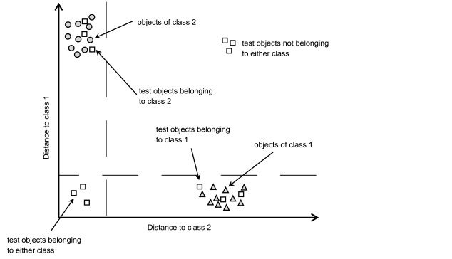
New objects are then classified based on the individual PCA models. A new object is projected into each of these models and assigned to a certain class when its residual distance from this model is below the limit for this class (Figure 5.21.-6). Distances of objects to the respective classes can be calculated by procedures such as either Euclidean or Mahalanobis distance. Consequently an object may belong to either 1 or multiple classes if the corresponding distances are within the required threshold. If the distance of an object to all of the SIMCA classes is above the threshold, then it will be classified as an outlier.

Figure 5.21.-6. – Plot representing the 4 possible classifications of test objects in a two-class SIMCA analysis (□ = unknown sample to classify, Δ = class 1 sample,○ = class 2 sample)

2-3-3 Critical aspects

Since SIMCA is mainly based on PCA principles, the validation of the method should follow that of PCA. In addition to this, the overlap of different classes must also be taken into account. For example, a molecule can have several chemical groups that appear in its spectroscopic profile. Thus, grouping such data into chemical subgroups results in overlap since separation is not possible.

2-3-4 Potential use

SIMCA is often used for the classification of analytical data from techniques such as near-infrared (NIR) or mass spectroscopy, and other analytical techniques such as chromatography and chemical imaging. SIMCA is more suitable than PCA for discriminating between classes that are difficult to separate.

2-4 CLUSTERING

2-4-1 Introduction

A cluster consists of a group of objects or data points similar to each other. Clustering tools can be used to visualise how data points ‘self-organise’ into distinct groups or to highlight the degree of similarity between data objects. Data points from a particular cluster share some common characteristics that differentiate them from those gathered in other clusters. Clusters are characterised using 3 main properties; size, shape and distance to the nearest cluster. Clustering is an unsupervised method of data analysis and is used either for explanatory or confirmatory analysis. It differs from discriminant analysis, which is a supervised classification technique, where an unlabelled object is assigned to a group of pre-classified objects.

2-4-2 Principle

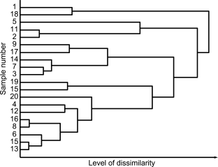
Numerous data clustering approaches are available and are typically classed as either hierarchical or non-hierarchical. Hierarchical clustering leads to the classical dendrogram graphical representation of the data, whereas non-hierarchical clustering finds clusters without imposing a hierarchical structure. Numerous algorithms are described in the literature, where data is partitioned either in a specific way or by optimising a particular clustering criterion. This simple and exclusive distinction is incomplete since mixed algorithms have similarities to both approaches. Hierarchical clustering recursively finds clusters either in agglomerative (bottom-up) or divisive (top-down) mode to form a tree shaped structure. Agglomerative mode starts with defining each data point as its own cluster and then merging similar clusters in pairs before repeating this step until the complete data set is classified (Figure 5.21.-7). Divisive mode starts by considering the entire data set as a single cluster, which is then recursively divided until only clusters containing a unique data point are obtained. Algorithms differ in the way they calculate the similarity between clusters. Complete link and single link algorithms calculate the distance between all pairs of objects that belong to different clusters in order to evaluate the similarity between them. In the single link method, this distance corresponds to the minimum distance separating 2 objects originating from 2 different clusters whereas in complete link algorithm this distance corresponds to the largest distance between 2 objects from 2 different clusters. Ward’s algorithm, also called the minimum variance algorithm, calculates the similarity between clusters by means of decreasing cluster variance when the 2 most similar clusters are merged.

Figure 5.21.-7. – Dendrogram for agglomerative hierarchical clustering until clusters containing a unique data point are obtained

Non-hierarchical clustering cannot be described and categorised as easily as hierarchical clustering. Different algorithms exist, which give rise to different classification schemes. An overview of the different categories of algorithms is given below ranging from simple distance based methods such as the minimum spanning tree and the nearest neighbour algorithms, to more sophisticated methods such as the K-means algorithm (often cited as a classical partition method), the expectation-maximisation algorithm (for ‘model-based’ methods) and DBSCAN for ‘density-based’ algorithms and, also, the ‘grid-based’ methods which are exemplified by the statistical information grid (STING) algorithm.

Minimum spanning tree clustering, such as Kruskal’s algorithm, is similar to the graph theory algorithm as all the data points are first of all connected by drawing a line between the closest points. When all data points are linked, the lines of largest length are broken, leaving clusters of closely connected points. For nearest neighbour clustering, an iterative procedure is used to assign a data point to a cluster when the distance between this point and its immediate neighbour (that belongs to a cluster) is below a pre-defined threshold value.

The K-means algorithm is one of the most popular and as with partition algorithms, the number of clusters must be chosen a priori, together with the initial position of the cluster centres. A squared error criterion measures the sum of the squared distance between each object and the centroid of its corresponding cluster. The K-means algorithm starts with a random initial partition and progresses by reassigning objects to clusters until the desired criteria reach a minimum. Some variants of the K-means algorithm allow the splitting or merging of clusters in order to find the optimum number of clusters, even when starting from an arbitrary initial clustering. Model-based clustering attempts to find the best fit for the data using a preconceived model. An example of this is the EM or expectation-maximisation algorithm, which assigns each object to a particular cluster according to the probability of membership for that object. In the EM algorithm, the probability function is a multivariate Gaussian distribution and that is iteratively adjusted to data by use of the maximum-likelihood estimation. The EM algorithm is considered as an extension of the K-means algorithm since the residual sum of squares used for K-means convergence is similar to the maximum-likelihood criterion.

Density-based (DB) clustering, such as the DBSCAN algorithm, assimilates clusters to regions of high density separated by regions of low or no density. The neighbourhood of each object is examined to determine the number of other objects that fit within a specified radius and a cluster is defined when a sufficient number of objects inhabit this neighbourhood.

Grid-based algorithms, such as STING, divide the data space into a finite number of cells. The distribution of objects within each cell is then computed in terms of mean, variance, minimum, maximum and type of distribution. There are several levels of cells, providing different levels of resolution and each cell of a particular level corresponds to the union of 4 child cells from the lower level.

2-4-3 Critical aspects

Algorithms are sensitive to the starting conditions used to initialise the clustering of data. For example, K-means needs a pre-set number of clusters and the resultant partitioning will vary according to the chosen number of clusters. The metrics used in distance calculation will also influence data clustering. For Euclidean distances, the K-means algorithm will define spherical clusters whereas they could be ellipsoidal when using Mahalanobis distances. The cluster shape can be modified by data pre-treatments prior to cluster analysis. DB algorithms can deal with arbitrarily shaped clusters, but their weakness is their limitation in handling high-dimensional data, where objects are sparsely distributed among dimensions.

When an object is considered to belong to a cluster with a certain probability, algorithms such as density based clustering, allow a soft or fuzzy clustering. In this case, the border region of 2 adjacent clusters can house some objects belonging to both clusters.

2-4-4 Potential use

Clustering is an exploratory method of analysis that helps in the understanding of data structure by grouping objects that share the same characteristics and in addition, hierarchical clustering allows for classification within data objects. Clustering is used in a vast variety of fields, in particular for information retrieval from large databases. For the latter, the term ‘data mining’ is frequently used, where the objective is to extract hidden and unexploited information from a large volume of raw data in search of associations, trends and relationships between variables.

2-5 MULTIVARIATE CURVE RESOLUTION

2-5-1 Introduction

Multivariate curve resolution (MCR) is related to principal components analysis (PCA) but, where PCA looks for directions that represent maximum variance and are mutually orthogonal, MCR strives to find contribution profiles (i.e. MCR scores) and pure component profiles (i.e. MCR loadings). MCR is also known as self-modelling curve resolution (SMCR) or end-member extraction. When optimising MCR parameters the alternating least squares (ALS) algorithm is commonly used.

2-5-2 Principle

MCR-ALS estimates the contribution profiles C and the pure component profiles S from the data matrix X, i.e. X = C∙S^T + E just as in classical least squares (CLS). The difference between CLS and ALS is that ALS is an iterative procedure that can incorporate information that is known about the physicochemical system studied and use this information to constrain the components/factors. For example, neither contribution nor absorbance can be negative by definition. This fact can be used to extract pure component profiles and contributions from a well-behaved data set. There are also other types of constraints that may be used, such as equality, unimodality, closure and mass balance.

It is often possible to obtain an accurate estimation of the pure component spectra or the contribution profiles and these estimates can then be used as initial values in the constrained ALS optimisation. New estimates of the profile matrix S and of the contribution profile C are obtained during each iteration. In addition, the physical and chemical knowledge of the system can be used to verify the result, and the resolved pure component contribution profiles should be explainable using existing knowledge. If the MCR results do not match the known system information, then other constraints may be needed.

2-5-3 Critical aspects

Selection of the correct number of components for the ALS calculations is important for a robust solution and a good estimate can be obtained using for example, evolving factor analysis (EFA) or fixed-size moving window EFA. Furthermore, the constraints can be set as either ‘hard’ or ‘soft’, where hard constraints are strictly enforced while soft constraints leave room for deviations from the restricted value. Generally, due to inherent ambiguities in the solution obtained, the MCR scores will need to be translated into, for example, the concentration of the active pharmaceutical ingredient, using a simple linear regression step. This means that the actual content must be known for at least 1 sample. When variations of 2 or more chemical entities are in some way correlated, rank deficiency occurs, for example 1 entity is formed while the other is consumed, or 2 entities are consumed at the same rate to yield a third. As a result, the variation of the individual substance is essentially masked and in such cases, simultaneous analysis of data from independent experiments using varied conditions or combined measurements from 2 measurement techniques generally results in better strategies than analysing the experiments separately one by one.

2-5-4 Potential use

MCR can be applied when the analytical method produces multivariate data for which the response is either linear or linearisable. This has the advantage that only 1 standard is needed per analyte, which is particularly beneficial when the measurements are at least partly selective between analytes. When linearity and selectivity is an issue, more standards per analyte may be required for calibration. When there is no pure analytical response for an analyte, it is also possible to estimate starting vectors by applying PCA to analyte mixtures together alongside varimax rotation of the PCA coordinate system. ALS implementations of MCR may also allow analyte profiles that are freely varied by the algorithm, which can then be used to model a profile that is difficult to estimate separately, for example a baseline.

2-6 MULTIPLE LINEAR REGRESSION

2-6-1 Introduction

Multiple Linear Regression (MLR) is a classical multivariate method that uses a combined set of x-vectors (X-data matrix) in linear combinations that are fitted as closely as possible to the corresponding single y-vector.

MLR extends linear regression to more than 1 selected variable in order to perform a calibration using least squares fit.

2-6-2 Principle

In MLR, a direct least squares regression is performed between the X- and the Y-data. For the sake of simplicity, the regression of only 1 column vector y will be addressed here, but the method can be readily extended to a Y-matrix, as is common when MLR is applied to data from experimental design (DoE), with multiple responses. In this case, single independent MLR models for each y-variable can be applied to the same X-matrix.

The following MLR model equation is an extension of the normal univariate straight line equation; it may also contain cross and square terms:

This can be compressed into the convenient matrix form:

The objective is to find the vector of regression coefficients b that best minimises the error term f. This is where the least squares criterion is applied to the squared error terms, i.e. to find b-values so that y-residuals f are minimised. MLR estimates the model coefficients using the following equation:

This operation involves the matrix inversion of the variance-covariance matrix (X^TX)^-1. If any of the X-variables show any collinearity with each other i.e. if the variables are not linearly independent, then the MLR solution will not be robust or a solution may not even be possible.

2-6-3 Critical aspects

MLR requires independent variables in order to adequately explain the data set, but as pharmaceutical samples are comprised of a complex matrix in which components interact to various degrees, the selection of appropriate variables is not straightforward. For example, in ultra-violet spectroscopy, observed absorbance values are linked because they may describe related behaviours in the spectroscopic data set. When observing the spectra of mixtures, collinearity is commonly found among the wavelengths, and consequently, MLR will struggle to perform a usable linear calibration.

The ability to vary the x-variables independently of each other is a crucial requirement when using variables as predictors with this method. This is why in DoE the initial design matrix is generated in such a way as to establish this independence (i.e. orthogonality) from the start. MLR has the following constraints and characteristics:

— the number of X-variables must be smaller than the number of samples (n>m), otherwise the matrix cannot be inverted;

— in case of collinearity among X-variables, the b-coefficients are not reliable and the model may be unstable;

— MLR tends to over-fit.

To avoid overfitting MLR is often used with variable selection.

The selection of the optimal number of X-variables can be based on their residual variance, but also on the prediction error.

2-6-4 Potential use

MLR is typically suited to simple matrices/data sets, where there is a high degree of specificity and full rank. As matrices become more complex, more suitable methods such as PLS may be required to provide more accurate and/or robust calibration. In these cases, MLR may be used as a screening technique prior to the application of more advanced calibration methodologies.

2-7 PRINCIPAL COMPONENTS REGRESSION

2-7-1 Introduction

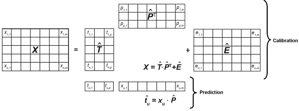
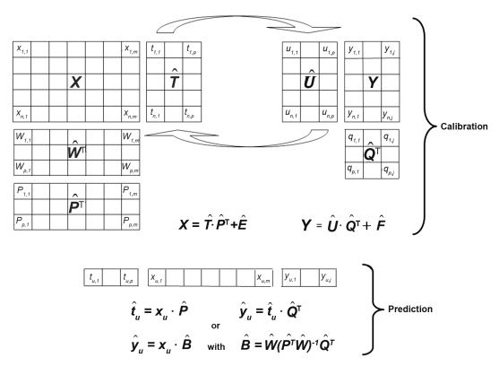
Principal components regression (PCR) is an expansion of principal components analysis (PCA) for use in quantitative applications. It is a two-step procedure whereby the calibration matrix X is first of all transformed by PCA into the scores and loadings matrices T̂ and P̂ respectively. In the following step, the score matrix for the principal components is used as the input for an MLR model to establish the relationship between the X- and the Y-data.

2-7-2 Principle

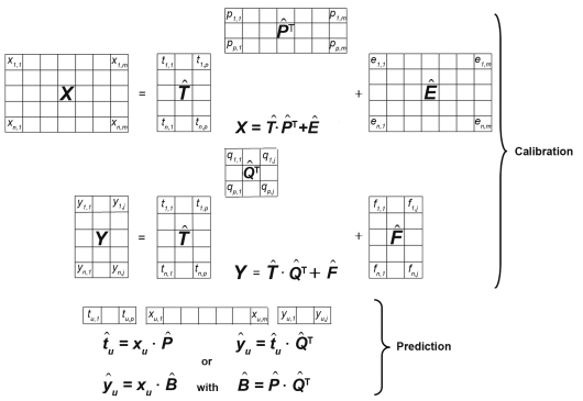
As in PCA, the calibration matrix is decomposed into scores and loadings matrices in such a way as to minimise the residual matrix Ê that ideally consists only of random errors, i.e. noise. For quantitative calibration, an additional matrix Y with the reference analytical data of the calibration samples is necessary. As the concentration information is contained in the orthogonal score vectors of the T̂-matrix it can be optimally correlated by multiple linear regression using the actual concentrations in the Y-matrix via the matrix Q̂ (Figure 5.21.-8), while minimising the entries in the residual matrix F̂.

Figure 5.21.-8. – Decomposition of the matrices for principal components regression (PCR)

2-7-3 Critical aspects

A crucial point in the development of a model is the selection of the optimal number of principal components. In this respect, the plot of the number of principal components versus the residual Y-variance is an extremely useful diagnostic tool when defining the optimal number of PCs, i.e. when the minimum of the residual Y-variance observed during model assessment has been reached. In most cases, additional PCs beyond this point do not improve the prediction performance but the calibration model falls into overfitting.

Despite its value as an important tool when dealing with collinear X-data, the weakness of PCR lies in its independent decomposition of the X and Y matrices. This approach may take into account variations of the X-data that are not necessarily relevant for an optimal regression with the Y-data. Also, Y-correlated information may even get lost in higher order principal components that are neglected in the above-mentioned selection process of the optimal number of PCs.

A stepwise principal component selection (e.g. selection of PC2 instead of PC1) may be useful to improve the performance of the calibration model.

2-7-4 Potential use

PCR is a multivariate technique with many diagnostic tools for the optimisation of the quantitative calibration models and the detection of erroneous measurements. In spectroscopy for example, PCR provides stable solutions when dealing with the calibration data of either complete spectra or large spectral regions. However, it generally requires more principal components than PLS and in view of the limitations and disadvantages discussed above, PLS regression has become the preferred alternative for quantitative modelling of spectroscopic data.

2-8 PARTIAL LEAST SQUARES REGRESSION

2-8-1 Introduction

Partial least squares regression (PLSR, generally known as PLS and alternatively named projection on latent structures) has developed into the most popular algorithm for multivariate regression.

PLS relates 2 data sets (X and Y) irrespective of collinearity. PLS finds latent variables from X and Y data blocks simultaneously, while maximising the covariance structure between these blocks. In a simple approximation PLS can be viewed as 2 simultaneous PCA analyses applied to the X and Y-data in such a way that the structure of the Y-data is used for the search of the principal components in the X-data. The amount of variance modelled, i.e. the explained part of the data, is maximised for each component. The non-explained part of the data set is made up of residuals, which function as a measure of the modelling quality.

2-8-2 Principle

The major difference between PCR and PLS regression is that the latter is based on the simultaneous decomposition of the X and Y-matrices for the derivation of the components (preferably denoted as PLS factors, factors, or latent-variables). Consequently, for the important factors, the information that describes a maximum variation in X, while correlating as much as possible with Y, is collected. This is precisely the information that is most relevant for the prediction of the Y-values of unknown samples. In practice PLS can be applied to either 1 Y-variable only (PLS1), or to the simultaneous calibration of several Y-variables (PLS2 model).

As the detailed PLS algorithms are beyond the scope of this chapter, a simplified overview is instead given (Figure 5.21.-9). Arrows have been included between the T̂ and Û scores matrices in order to symbolise the interaction of their elements in the process of this iteration. While the Y-matrix is decomposed into the loadings and scores matrices Q̂ and Û respectively, the decomposition of the X-matrix produces not only the loadings and scores matrices P̂ and T̂, but also a loading weights matrix Ŵ, which represents the relationship between the X and Y-data.

To connect the Y-matrix with the X-matrix decomposition for the first estimation of the T̂ score values, the Y-data are used as a guide for the decomposition of the X-matrix. By interchanging the score values of the Û and T̂ matrices, an interdependent modelling of the X and Y data is achieved, thereby reducing the influence of large X-variations that do not correlate with Y. Furthermore, simpler calibration models with fewer PLS-factors can also be developed where, as is the case for PCR, residual variances are used during validation to determine the optimal number of factors that model useful information and consequently, avoid overfitting.

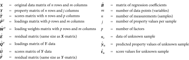
Figure 5.21.-9. – Decomposition of the data matrices for PLS regression

2-8-3 Critical aspects

A critical step in PLS is the selection of the number of factors. Selecting too few factors will inadequately explain variability in the training data set, while too many factors will cause overfitting and instability in the resulting calibration (Figure 5.21.-10). The optimal number of factors is estimated during validation of the calibration. Figure 5.21.-10 shows the changes in the calibration error (A) of a model and 2 cases of prediction errors (B, C) according to the number of factors used in the model. The calibration error decreases continuously as the number of factors increases. In case B prediction error reveals that no minimum can be observed; however, a minimum is observed in case C. In the absence of a minimum, the number of components can be chosen based on where no significant decreasing of error is observed.

As far as the decision between PLS1 or PLS2 models is concerned PLS1 modelling is chosen if there is only 1 Y-variable of interest. In cases where there is more than 1 Y-variable of interest, either one PLS2 model or individual PLS1 models for each Y-variable can be calculated. In general, PLS2 is the preferred approach for screening purposes and in cases of highly correlated Y-variables of interest; otherwise separate PLS1 models for the different Y-variables will yield more satisfactory prediction results.

2-8-4 Potential use

PLS has emerged as a preferable alternative to PCR for quantitative calibration because it incorporates the intervention of the Y-data structure for the decomposition of the calibration X-matrix. Consequently, information from the most important factors is collected and is capable of describing maximal variation in the X-data, while also correlating as closely as possible with the Y-data. In general, this yields simpler models with fewer factors compared to PCR and also provides superior interpretation possibilities and visualisation diagnostics for the optimisation of the calibration performance. In addition PLS can handle presence of noise in both X- and Y-data.

PLS discriminant analysis (PLS-DA) is a special case of PLS where X-matrix is regressed into a dummy Y-matrix consisting of ones and zeroes. Ones and zeroes indicate the class to which samples are belonging or not. PLS-DA is used as a semi-quantitative method in, for example, chemical imaging estimating the pixel components.

Figure 5.21.-10. – Effects of adding factors to a model; the calibration becomes more accurate i.e. the residual error diminishes, while the predictive performance of the model could deteriorate as for prediction C. The optimum number of factors reflects a compromise

2-9 SUPPORT VECTOR MACHINES

2-9-1 Introduction

To achieve classification, multivariate techniques reduce the dimensionality and complexity of the data set. Kernel methods project data into higher dimensional feature spaces.

2-9-2 Principle

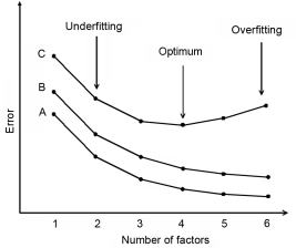
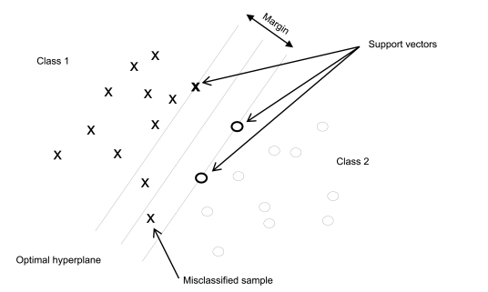
Support vector machines (SVMs) project X-data of the training set into a feature space of usually much higher dimension than the original data space. In the feature space a hyperplane (also called decision plane) is computed that separates individual points of known group membership (Figure 5.21.-11). The best discriminating separation is achieved by maximising the margin between groups. The margin is defined by 2 parallel hyperplanes at an equal distance from the decision plane. The optimum position of the decision plane is obtained if the margin is maximal. Points in the feature space that define the margin are called support vectors.

For each training point the distance to the decision plane is computed. In the case of a two-class separation for example, the sign of the distance gives the group membership and the value corresponds to the certainty of classification. During modelling the distance between the training points and the hyperplane contributes to the weight attributed to the point. Very distant points will have a lesser weight, and to avoid overfitting, distances smaller than a trade-off parameter will not be considered.

For non-separable object groups overlapping is allowed to a certain extent. So-called slack variables are added to objects, with value 0 if correctly classified and a positive value otherwise. The optimal hyperplane is found by maximising the margin at the same time allowing for a minimum number of training points to be misclassified (Figure 5.21.-12). The proportion of misclassified points becomes a control parameter during margin maximisation.

Figure 5.21.-11. – The object space, where separation of the 2 classes is not possible, is mapped into a feature space where separation is possible

In practice SVM computation is extremely complex and would be infeasible without simplifying of the optimisation problem. To project X-data into the feature space the original data is expanded by a set of basis functions. Selecting particular basis functions makes it possible to reformulate the whole optimisation procedure. Only products of the expanded variables remain part of the optimisation procedure and they can be advantageously replaced by a Kernel function.

Figure 5.21.-12. – In the feature space, the separation of classes 1 and 2 was achieved with toleration of certain misclassified samples

2-9-3 Critical aspects

Numerous algorithms and different types of software can be used to compute SVMs, which may lead to differing results. Optimisation will vary depending on the algorithm used. Control criteria may differ, thus leading either to divergence during the iterations, or to unstable computations sensitive to redundant and uninformative data.

During SVM computation training points that are well inside their class boundaries have little or even no effect on the position of the decision plane. The latter focusses mainly on points that are difficult to separate and not on objects that are clearly distinct. Thus, SVMs are sensitive to redundant values and atypical points like outliers, for example. As a consequence it may be pertinent to select or screen out specific variables prior to performing SVM. The data should be normalised and standardised to avoid having input data of different scales, which may lead to poor conditions for the boundary optimisation.

The best performing model must be adequately validated and test data that is completely untouched during iterations is required for this purpose. It should be ensured that this data is well balanced in the sense that both easy and difficult samples are equally represented in the training and validation sets.

2-9-4 Potential use

SVMs are mainly used for binary supervised classification. They can be generalised to multiclass classification or extended to regression problems, though these applications are not considered within the scope of this chapter. Objects that are difficult to classify rather than those that are clearly distinct drive the optimisation process in SVMs. SVMs can be used for the separation of classes of objects, but not for the identification of these objects. They operate well on large data sets that are obtained, for example, by NIR spectroscopy, magnetic resonance, chemical imaging or process data mining, where PCA and related methods fail. Their strength mainly lies in separation of samples featuring highly correlated signals, i.e. polymorphs, excipients, tracing of adulterated substances, counterfeits etc.

2-10 ARTIFICIAL NEURAL NETWORKS

2-10-1 Introduction

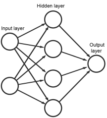
Artificial neural networks (ANNs) are general computational tools, whose initial development was inspired by the need for further understanding of biological neural networks and which have since been widely used in various areas that require data processing with computers or machines. The methods for building ANN models and their subsequent applications can be dramatically different depending on the architecture of the neural networks themselves. In the field of chemometrics, ANNs are generally used for multivariate calibration and unsupervised classification, which is achieved by using multi-layer feed-forward (MLFF) neural networks, or self-organising maps (SOM) respectively. As a multivariate calibration tool, ANNs are more generally associated with the mapping of non-linear relationships.

2-10-2 Principle

2-10-2-1 General

The basic data processing element in an artificial neural network is the artificial neuron, which can be understood as a mathematical function that uses the sum of a weighted vector and a bias as the input. The vector is the ‘input’ of the neuron and is obtained either directly from a sample in the data set or calculated from previous neurons. The user chooses the form of the function (called transfer function). The weights and bias are the coefficients of the ANN model and are determined through a learning process using known examples. An ANN often contains many neurons arranged in layers, where the neurons in each layer are arranged in parallel. They are connected to neurons in the preceding layer from which they receive inputs and also to neurons in the following layer where the outputs are sent (Figure 5.21.-13). The output of 1 neuron is therefore used as the input for neurons in the following layer. The input layer is a special layer that receives data directly from the user and sends this information directly to the next layer without applying a transfer function. The output layer is similar in that its output is also directly used as the model output without any additional processing. The unlimited possibilities when connecting different numbers and layers of neurons, is often called an ANN architecture, and provides the potential for ANNs to meet any complicated data modelling requirements.

Figure 5.21.-13. - Typical arrangements of neuron layers and their inter-connections

2-10-2-2 Multi-layer feed-forward artificial neural network

A multi-layer feed-forward network (MLFF ANN) contains an input layer, an output layer and 1 or more layers of neurons in-between called hidden layers. Even though there is no limit on how many hidden layers may be included, an MLFF ANN with only 1 hidden layer is sufficiently capable of handling most multivariate calibration tasks in chemometrics. In an MLFF ANN, each neuron is fully connected to all the neurons in the neighbouring layers. A hyperbolic tangent sigmoid transfer function is usually used in MLFF ANN, but other transfer functions, including linear functions, can also be used.

The initial weights and biases can be set as small random numbers, but can also be initialised using other algorithms. The most popular training algorithm for determining the final weights and biases is the back-propagation (BP) algorithm or its related variants. In the BP algorithm, the prediction error, calculated as the difference between the ANN output and the actual value, is propagated backward to calculate the changes needed to adjust the weights and biases in order to minimise the prediction error.

An MLFF ANN must be optimised in order to achieve acceptable performance. This often involves a number of considerations including the number of layers, the number of neurons in each layer, transfer functions for each layer or neuron, initialisation of weights, learning rate, etc.

2-10-2-3 Self-organising map

The aim of the self-organising map (SOM) is to create a map where observations that are close to each other have more similar properties than more distant observations. The neurons in the output layer are usually arranged in a two-dimensional map, where each neuron can be represented as a square or a hexagon. SOMs are trained using competitive learning that is different from the above described method using BP. The final trained SOM is represented as a two-dimensional map of properties.

2-10-3 Critical aspects

The 2 most common pitfalls of using ANNs are over-training and under-training. Over-training means that an ANN model can predict the training set very well but ultimately fails to make good predictions. Under-training means that the ANN training ended too soon and therefore the resultant ANN model underperforms when making predictions. Both of these pitfalls should be avoided when using ANNs for calibration. A representative data set with a proper size, i.e. more observations or samples than variables, is required before a good ANN model can be trained. Generally, since the models are non-linear, more observations are needed than for a comparable data set subjected to linear modelling. As for other multivariate calibration methods, the input may need pre-processing to balance the relative influence of variables. One advantage of pre-processing is the reduction in the number of degrees of freedom of input to the ANN, for example by compression of the X-data to scores by PCA and then using the resulting scores for the observations as input.

2-10-4 Potential use

The advantage of MLFF ANN in multivariate calibration lies in its ability to model non-linear relationships. Since the neurons are fully connected, all the interactions between variables are automatically considered. It has been proven that a MLFF ANN with sufficient hidden neurons can map any complicated relationship between the inputs and outputs.

SOMs can be used to visualise high-dimensional data while preserving the topology in the original data. They are based on unsupervised learning, and are mainly useful as tools to explore features in data sets where no prior knowledge of the patterns and relationships of the samples exists.

The ANNs often have a large number of coefficients (weights and biases) that give the ANN the potential to model any complicated relationships in the data set but as a result, can also make the interpretation of the coefficients more difficult. However, when linear modelling methods are not flexible enough to provide the required prediction or classification accuracy, ANNs may be a good alternative.

3 GLOSSARY

β-distribution

Continuous probability distribution with density function

where u > 0, v > 0 are shape parameters (degrees of freedom) and B is the beta function,

The γ-quantile of the Β(u,v)-distribution is denoted by β_u,v;γ and it is the value q such that the value of the distribution function F is γ:

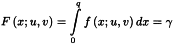
Bootstrapping

A number of sample sets of size n that is produced from an original sample set of the same size n by means of a random selection of samples with replacement.

Centring

A data set is mean centred by calculating the mean value of each variable and subtracting the variable mean values from each column of variables, in order to make the comparison and interpretation of the data easier.

Collinear/non-collinear

A family of vectors is collinear if at least 1 of the vectors can be represented as a linear combination of the other vectors. Hence a family of vectors is non-collinear if none of the vectors can be represented as a linear combination of the others.

Component (or factor, latent variable)

In chemometrics: underlying, non-observed, non-measured, hypothetical variable that contributes to the variance of a collection of measured variables. The variables are linear combinations of the factors and these factors are assumed to be uncorrelated with each other.

Data mining

Process of exploration, extraction and modelling of large collections of data in order to discover a priori unknown relationships or patterns.

Dependent variable

Also a response, regressand: a variable that is related by a formal (explicit) or empirical mathematical relationship to 1 or more other variables (typically the Y-data).

Empirical model

A data-driven model established without assuming an explicit mathematical relationship, or without a description of the behaviour of a system based on accepted laws of physics.

Exploratory data analysis

The process for uncovering unexpected or latent patterns in order to build future hypotheses.

Factor

See component.

Hotelling T² statistics

Multivariate version of the t-statistic. In general, this statistic can be used to test if the mean vector of a multivariate data set has a certain value or to compare the means of the variables. The T² statistic is also used for detection of outliers in multivariate data sets. A multivariate statistical test using the Hotelling T² statistic can be done. A confidence ellipse can be included in score plots to reveal points outside the ellipse as potential outliers.

Independent variable

Input variable on which other variables are dependent through a mathematical relationship (typically the X-data).

Indirect prediction

Process for estimating the value of a response on the basis of a multivariate model and observed data.

Interference

Effect of substances, physical phenomena or instrument artefacts, separate from the target analyte, that can be measured by the chosen analytical method. Then there is a risk of confusion between the analyte and interference if the interference is not varied independently or at least randomly in relation to the analyte.

Latent variable

See component.

Leave-one-out

In a ‘leave-one-out’ procedure only 1 sample at a time is removed from the data set in order to create a new data set.

Leave-subset-out

In a ‘leave-subset-out’ procedure a subset of samples is removed from the data set in order to create a new data set.

Leverage

A measure of how extreme a data point or a variable is compared to the majority. Points or variables with a high leverage are likely to have a large influence on the model.

Loadings

Loadings are estimated when information carried by several variables is focussed onto a few components. Each variable has a loading alongside each model component. The loadings show how well a variable is taken into account by the model components.

Orthogonal

2 vectors are orthogonal if their scalar product is 0.

Orthonormal vectors

Orthogonal and normalised (unit-length) vectors.

Outlier

For a numerical data set, it relates to a value statistically different from the rest. Also refers to the sample associated with that value. Specific statistical testing for outliers may be used.

Overfitting

For a model, overfitting is a tendency to describe too much of the variation in the data, so that in addition to the consistent underlying structure, some noise or non-informative variation is also taken into account and unreliable predictions will be obtained.

Property

See variable.

Resampling

The process of impartial rearrangement and sub-sampling of the original data set. This occurs during optimisation/validation procedures that repeatedly calculate a property and the error associated with it. Typical examples are cross-validation and bootstrapping, which create successive evaluation data sets by repeated sub-sampling.

Reselection

Reuse of samples (see resampling).

Residuals

A measure of the variation that is not taken into account by the model or a deviation between predicted and reference values.

Root mean square error of prediction

A function of the predictive residual sum of squares to estimate the accuracy:

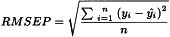
where ŷ_i is the predicted response for the i^th sample of the test data set and y_i the observed response of the i^th sample, and n is the number of samples.

Sample

Object, observation, or individual from which data values are collected.

Sample attribute

Qualitative or quantitative property of the sample.

Sample selection

The process of drawing a subset or a collection from a population in order to estimate the properties of the population.

Scores or factor score coefficients

Coordinates of the samples in the new coordinate system defined by the principal components. Scores represent how samples are related to each other’s given the measurement variables.

Score (normalised)

j^th score value t_i,j of the i^th sample divided by the norm of the scores matrix:

where p is the number of parameters in the model.

Standard error of calibration

A function of the predictive residual sum of squares to estimate the accuracy considering the number of parameters:

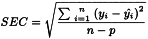
where n is the number of samples of the learning set, p the number of parameters in the model to be estimated by using the sample data, ŷ_i the i^th fitted value in the calibration, and y_i the i^th reference value. In multiple regression with m variables p = m + 1 (1 coefficient for each of the m variables and 1 intercept).

Standard error of laboratory

Concerns to the intermediate precision or reproducibility, whichever is applicable.

Supervised

Refers to modelling data labelled by classes or values.

Unsupervised (non-supervised)

Refers to exploring data without prior assumptions.

Underfitting

The reverse of overfitting.

Variable

Property of a sample that can be assessed (attribute, descriptor, feature, property, characteristics).

Varimax rotation

Orthogonal analytical rotation of factors that maximises the variance of squared factor loadings, thereby increasing the large factor loadings and large eigenvalues and decreasing the small ones in each factor.

4 ABBREVIATIONS

ALS	alternating least squares
ANN	artificial neural network
BP	back-propagation
CLS	classical least squares
DB	density-based
DBSCAN	density-based spatial clustering of applications with noise
DoE	design of experiments
EFA	evolving factor analysis
EM	expectation maximisation
LDA	linear discriminant analysis
MCR	multivariate curve resolution
MLFF	multi-layer feed-forward
MLR	multiple linear regression
MSPC	multivariante statistical process control
NIR	near infrared
PAT	process analytical technology
PC	principle component
PCA	principal components analysis
PCR	principal components regression
PLS	partial least squares regression
PLS-DA	partial least squares discriminant analysis
PLSR	partial least squares regression
QbD	quality by design
QDA	quadratic discriminant analysis
RMSEP	root mean square error of prediction
SEC	standard error of calibration
SEL	standard error of laboratory
SIMCA	soft independent modelling of class analogy
SMCR	self-modelling curve resolution
SNV	standard normal variate
SOM	self-organising map
STING	statistical information grid
SVM	support vector machine